Loading data
We provide a simple guide in how to load your own data and initialize the adata object for downstream analysis. This tutorial assumes that the files are either in txt or mtx format. After running this pipeline, please see the folder test_data for how exactly each data is stored.
The first step to use CoSpar is to construct an anndata object that stores all relevant data. The key annotations after initialization are:
adata.X: state count matrix, shape (n_cell, n_gene). This should not be log-normalized.
adata.var_names: list of gene names, shape (n_genes,).
adata.obs[‘time_info’]: time annotation (type:
str) for each cell, shape (n_cell,).adata.obs[‘state_info’]: state annotation for each cell, shape (n_cell, 1). [Optional. Can be generated in preprocessing.
adata.obsm[‘X_clone’]: clonal labels for each cell in the form of np.array or sparse matrix, shape (n_cell, n_clone).
adata.obsm[‘X_pca’]: PCA matrix, shape (n_cell, n_pcs). [Optional. Can be generated in preprocessing.
adata.obsm[‘X_emb’]: two-dimensional embedding, shape (n_cell, 2). [Optional. Can be generated in preprocessing.
cs.pp.initialize_adata_object assists this initialization.
[1]:
import cospar as cs
import pandas as pd
import scipy.io as sio
import numpy as np
import os
[2]:
cs.logging.print_version()

# Set the messaging level. At a given value, a running function will
# print information at or below its level.
cs.settings.verbosity = 2  # range: 0 (error),1 (warning),2 (info),3 (hint).

# Plot setting. If you want to control a particular plot,
# just change the setting here, and run that plotting function.
cs.settings.set_figure_params(
    format="png", figsize=[4, 3.5], dpi=75, fontsize=14, pointsize=3
)
Running cospar 0.3.0 (python 3.8.16) on 2023-07-14 12:10.
ERROR: XMLRPC request failed [code: -32500]
RuntimeError: PyPI no longer supports 'pip search' (or XML-RPC search). Please use https://pypi.org/search (via a browser) instead. See https://warehouse.pypa.io/api-reference/xml-rpc.html#deprecated-methods for more information.
Each dataset should have its folder to avoid conflicts.
[3]:
# set the directory for figures and data. If not existed yet, they will be created automtaically.
cs.settings.data_path = "test_data"  # This name should be exactly 'text_data'
cs.settings.figure_path = "fig_cospar"
cs.hf.set_up_folders()

cs.datasets.raw_data_for_import_exercise()  # download the data
try downloading from url
https://github.com/ShouWenWang-Lab/cospar/files/12036732/test_data.zip
... this may take a while but only happens once
Import method A
Assuming that the X_clone data is stored in mtx format
[4]:
df_cell_id = pd.read_csv(os.path.join(cs.settings.data_path, "cell_id.txt"))
df_cell_id.head()
[4]:
| Cell_ID | |
|---|---|
| 0 | cell_10 |
| 1 | cell_13 |
| 2 | cell_18 |
| 3 | cell_32 |
| 4 | cell_70 |
[5]:
df_gene = pd.read_csv(os.path.join(cs.settings.data_path, "gene_names.txt"))
df_gene.head()
[5]:
| gene_names | |
|---|---|
| 0 | 0610009L18Rik |
| 1 | 0610037L13Rik |
| 2 | 1110012L19Rik |
| 3 | 1110020A21Rik |
| 4 | 1110028F11Rik |
[6]:
df_time = pd.read_csv(os.path.join(cs.settings.data_path, "time_info.txt"))
df_time.head()
[6]:
| time_info | |
|---|---|
| 0 | 6 |
| 1 | 6 |
| 2 | 6 |
| 3 | 6 |
| 4 | 6 |
[7]:
RNA_count_matrix = sio.mmread(
    os.path.join(cs.settings.data_path, "gene_expression_count_matrx.mtx")
)
RNA_count_matrix
[7]:
<781x2481 sparse matrix of type '<class 'numpy.float64'>'
        with 225001 stored elements in COOrdinate format>
[8]:
X_clone = sio.mmread(os.path.join(cs.settings.data_path, "cell_by_clone_matrx.mtx"))
X_clone
[8]:
<781x339 sparse matrix of type '<class 'numpy.int64'>'
        with 781 stored elements in COOrdinate format>
[9]:
df_state = pd.read_csv(os.path.join(cs.settings.data_path, "state_info.txt"))
df_state.head()
[9]:
| state_info | |
|---|---|
| 0 | Neutrophil |
| 1 | Baso |
| 2 | Monocyte |
| 3 | Monocyte |
| 4 | Baso |
[10]:
df_X_emb = pd.read_csv(os.path.join(cs.settings.data_path, "embedding.txt"))
df_X_emb.head()
[10]:
| x | y | |
|---|---|---|
| 0 | 1165.708 | -2077.047 |
| 1 | -980.871 | -2055.629 |
| 2 | 2952.953 | 281.797 |
| 3 | 1314.821 | -560.760 |
| 4 | -1067.502 | -1275.488 |
[11]:
X_emb = np.array([df_X_emb["x"], df_X_emb["y"]]).T
Now, initialize the adata object
[12]:
adata_orig = cs.pp.initialize_adata_object(
    X_state=RNA_count_matrix,
    gene_names=df_gene["gene_names"],
    cell_names=df_cell_id["Cell_ID"],
    time_info=df_time["time_info"],
    X_clone=X_clone,
    state_info=df_state["state_info"],
    X_emb=X_emb,
    data_des="my_data",
)
Create new anndata object
WARNING: X_pca not provided. Downstream processing is needed to generate X_pca before computing the transition map.
Time points with clonal info: ['2' '4' '6']
WARNING: Default ascending order of time points are: ['2' '4' '6']. If not correct, run cs.hf.update_time_ordering for correction.
WARNING: Please make sure that the count matrix adata.X is NOT log-transformed.
/Users/shouwen/Documents/packages/cospar/cospar/preprocessing/_preprocessing.py:96: FutureWarning: X.dtype being converted to np.float32 from float64. In the next version of anndata (0.9) conversion will not be automatic. Pass dtype explicitly to avoid this warning. Pass `AnnData(X, dtype=X.dtype, ...)` to get the future behavour.
  adata = sc.AnnData(ssp.csr_matrix(X_state))
Update the time ordering. A correct time ordering is assumed later.
[13]:
cs.hf.update_time_ordering(adata_orig, updated_ordering=["2", "4", "6"])
[14]:
adata_orig
[14]:
AnnData object with n_obs × n_vars = 781 × 2481
    obs: 'time_info', 'state_info'
    uns: 'data_des', 'time_ordering', 'clonal_time_points'
    obsm: 'X_clone', 'X_emb'
Alternatively, you can initialize the object by building on an existing adata object. This will keep existing annotations from the old adata. You can make modifications by specifying additional entries.
[15]:
adata_orig_new = cs.pp.initialize_adata_object(adata=adata_orig, X_clone=X_clone)
WARNING: X_pca not provided. Downstream processing is needed to generate X_pca before computing the transition map.
Time points with clonal info: ['2' '4' '6']
WARNING: Default ascending order of time points are: ['2' '4' '6']. If not correct, run cs.hf.update_time_ordering for correction.
WARNING: Please make sure that the count matrix adata.X is NOT log-transformed.
[16]:
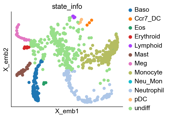
cs.pl.embedding(adata_orig, color="state_info")

Import method B
Assuming that the X_clone data is stored in a (cell_id, barcode_id) format
First, initialize the adata without concerning the clonal data
[17]:
df_cell_id = pd.read_csv(os.path.join(cs.settings.data_path, "cell_id.txt"))
df_gene = pd.read_csv(os.path.join(cs.settings.data_path, "gene_names.txt"))
df_time = pd.read_csv(os.path.join(cs.settings.data_path, "time_info.txt"))
RNA_count_matrix = sio.mmread(
    os.path.join(cs.settings.data_path, "gene_expression_count_matrx.mtx")
)
df_state = pd.read_csv(os.path.join(cs.settings.data_path, "state_info.txt"))
df_X_emb = pd.read_csv(os.path.join(cs.settings.data_path, "embedding.txt"))
X_emb = np.array([df_X_emb["x"], df_X_emb["y"]]).T
[18]:
adata_orig = cs.pp.initialize_adata_object(
    X_state=RNA_count_matrix,
    gene_names=df_gene["gene_names"],
    cell_names=df_cell_id["Cell_ID"],
    time_info=df_time["time_info"],
    state_info=df_state["state_info"],
    X_emb=X_emb,
    data_des="my_data",
)
Create new anndata object
WARNING: X_pca not provided. Downstream processing is needed to generate X_pca before computing the transition map.
Time points with clonal info: []
WARNING: Default ascending order of time points are: ['2' '4' '6']. If not correct, run cs.hf.update_time_ordering for correction.
WARNING: Please make sure that the count matrix adata.X is NOT log-transformed.
/Users/shouwen/Documents/packages/cospar/cospar/preprocessing/_preprocessing.py:96: FutureWarning: X.dtype being converted to np.float32 from float64. In the next version of anndata (0.9) conversion will not be automatic. Pass dtype explicitly to avoid this warning. Pass `AnnData(X, dtype=X.dtype, ...)` to get the future behavour.
  adata = sc.AnnData(ssp.csr_matrix(X_state))
Now, load the clonal data. Here, we start with a table of (cell_id, clone_id) pair. The cell_id does not need to be ranked. It should match the cell_id in the adata_orig.obs_names
[19]:
df_X_clone = pd.read_csv(
    os.path.join(cs.settings.data_path, "clonal_data_in_table_format.txt")
)
df_X_clone
[19]:
| Cell_ID | Clone_ID | |
|---|---|---|
| 0 | cell_0 | clone_275 |
| 1 | cell_1 | clone_329 |
| 2 | cell_2 | clone_56 |
| 3 | cell_3 | clone_236 |
| 4 | cell_4 | clone_213 |
| ... | ... | ... |
| 776 | cell_776 | clone_196 |
| 777 | cell_777 | clone_239 |
| 778 | cell_778 | clone_259 |
| 779 | cell_779 | clone_217 |
| 780 | cell_780 | clone_259 |
781 rows × 2 columns
[20]:
adata_orig.obs_names
[20]:
Index(['cell_10', 'cell_13', 'cell_18', 'cell_32', 'cell_70', 'cell_80',
       'cell_90', 'cell_97', 'cell_108', 'cell_117',
       ...
       'cell_7389', 'cell_7392', 'cell_7402', 'cell_7407', 'cell_7409',
       'cell_7417', 'cell_7423', 'cell_7435', 'cell_7436', 'cell_7437'],
      dtype='object', length=781)
[21]:
cs.pp.get_X_clone(adata_orig, df_X_clone["Cell_ID"], df_X_clone["Clone_ID"])
100%|███████████████████████████████████████| 87/87 [00:00<00:00, 412321.41it/s]
reorder clones
[22]:
adata_orig
[22]:
AnnData object with n_obs × n_vars = 781 × 2481
    obs: 'time_info', 'state_info'
    uns: 'data_des', 'time_ordering', 'clonal_time_points', 'clone_id'
    obsm: 'X_clone', 'X_emb'
[23]:
cs.pl.embedding(adata_orig, color="state_info")
[ ]: