Synthetic bifurcation

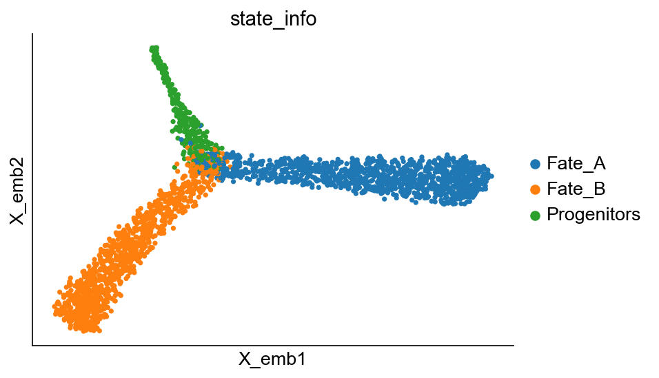
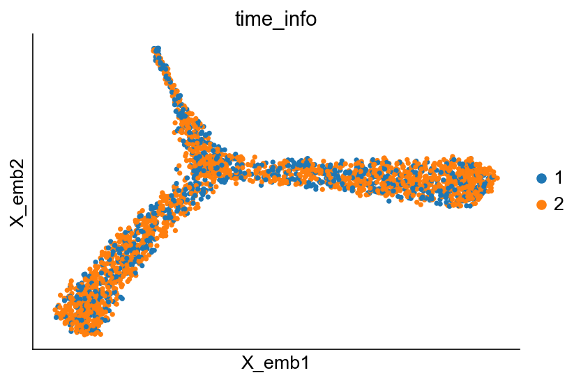
We simulated a differentiation process over a bifurcation fork. In this simulation, cells are barcoded in the beginning, and the barcodes remain un-changed. In the simulation we resample clones over time. The first sample is obtained after 5 cell cycles post labeling. The dataset has two time points. See Wang et al. (2021) for more details.

import cospar as cs

cs.logging.print_version()
cs.settings.verbosity = 2
cs.settings.set_figure_params(
    format="png", dpi=75, fontsize=14
)  # use png to reduce file size.

Running cospar 0.2.0 (python 3.8.12) on 2022-02-07 22:07.

cs.settings.data_path = (
    "test"  # A relative path to save data. If not existed before, create a new one.
)
cs.settings.figure_path = (
    "test"  # A relative path to save figures. If not existed before, create a new one.
)

Loading data

adata_orig = cs.datasets.synthetic_bifurcation()

adata_orig.obsm["X_clone"]

<2474x52 sparse matrix of type '<class 'numpy.float64'>'
        with 2474 stored elements in Compressed Sparse Row format>

cs.pl.embedding(adata_orig, color="state_info")

cs.pl.embedding(adata_orig, color="time_info")

Basic clonal analysis

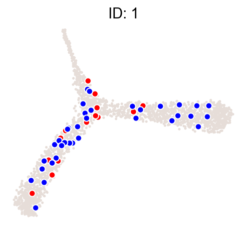
cs.pl.clones_on_manifold(adata_orig, selected_clone_list=[1])

cs.tl.fate_coupling(adata_orig, source="X_clone",normalize=False)
cs.pl.fate_coupling(adata_orig, source="X_clone")

Results saved as dictionary at adata.uns['fate_coupling_X_clone']

<AxesSubplot:title={'center':'source: X_clone'}>

cs.pl.barcode_heatmap(adata_orig, selected_times="2", color_bar=True, binarize=True)

Data saved at adata.uns['barcode_heatmap']

<AxesSubplot:>

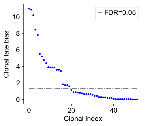
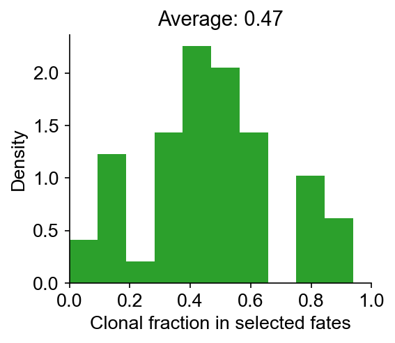
cs.tl.clonal_fate_bias(adata_orig, selected_fate="Fate_A", alternative="two-sided")
cs.pl.clonal_fate_bias(adata_orig)

100%|██████████| 52/52 [00:00<00:00, 254.70it/s]

Data saved at adata.uns['clonal_fate_bias']

Transition map inference

Transition map from multiple clonal time points.

adata = cs.tmap.infer_Tmap_from_multitime_clones(
    adata_orig,
    clonal_time_points=["1", "2"],
    smooth_array=[10, 10, 10],
    CoSpar_KNN=20,
    sparsity_threshold=0.2,
)

------Compute the full Similarity matrix if necessary------
----Infer transition map between neighboring time points-----
Step 1: Select time points
Number of multi-time clones post selection: 52
Step 2: Optimize the transition map recursively
Load pre-computed similarity matrix
Iteration 1, Use smooth_round=10
Iteration 2, Use smooth_round=10
Iteration 3, Use smooth_round=10
Convergence (CoSpar, iter_N=3): corr(previous_T, current_T)=0.96
-----------Total used time: 1.4379048347473145 s ------------

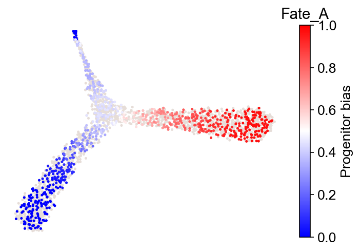
cs.tl.fate_bias(adata, selected_fates=["Fate_A", "Fate_B"], source="transition_map")
cs.pl.fate_bias(adata, source="transition_map")

Results saved at adata.obs['fate_map_transition_map_XXX']
Results saved at adata.obs['fate_bias_transition_map_fateA*fateB']
selected_fates not specified. Using the first available pre-computed fate_bias

Transition map from a single clonal time point

adata = cs.tmap.infer_Tmap_from_one_time_clones(
    adata_orig,
    initial_time_points=["1"],
    later_time_point="2",
    initialize_method="OT",
    smooth_array=[10, 10, 10],
    sparsity_threshold=0.2,
    compute_new=False,
)

Trying to set attribute `.uns` of view, copying.
Trying to set attribute `.uns` of view, copying.

--------Infer transition map between initial time points and the later time one-------
--------Current initial time point: 1--------
Step 0: Pre-processing and sub-sampling cells-------
Step 1: Use OT method for initialization-------
Load pre-computed shortest path distance matrix
Compute new custom OT matrix
Use uniform growth rate
OT solver: duality_gap
Finishing computing optial transport map, used time 3.3392720222473145
Step 2: Jointly optimize the transition map and the initial clonal states-------
-----JointOpt Iteration 1: Infer initial clonal structure
-----JointOpt Iteration 1: Update the transition map by CoSpar
Load pre-computed similarity matrix
Iteration 1, Use smooth_round=10
Iteration 2, Use smooth_round=10
Iteration 3, Use smooth_round=10
Convergence (CoSpar, iter_N=3): corr(previous_T, current_T)=0.98
Convergence (JointOpt, iter_N=1): corr(previous_T, current_T)=0.094
Finishing Joint Optimization, used time 1.3652610778808594
-----------Total used time: 4.814281940460205 s ------------

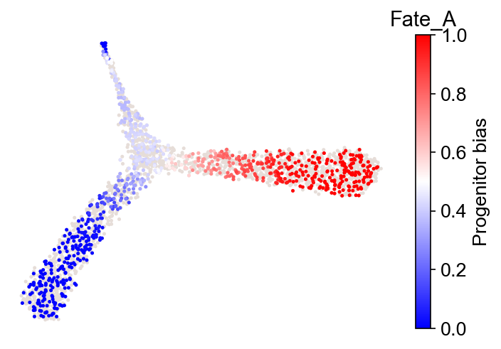
cs.tl.fate_bias(adata, selected_fates=["Fate_A", "Fate_B"], source="transition_map")
cs.pl.fate_bias(adata, source="transition_map")

Results saved at adata.obs['fate_map_transition_map_XXX']
Results saved at adata.obs['fate_bias_transition_map_fateA*fateB']
selected_fates not specified. Using the first available pre-computed fate_bias

Transition amp from only the clonal information

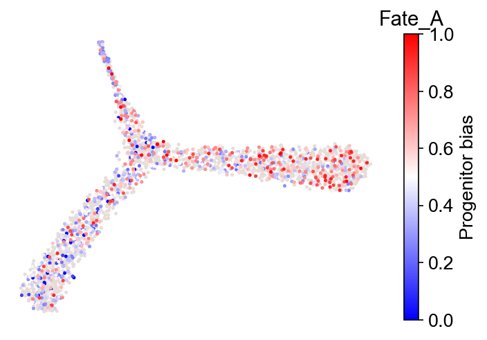
adata = cs.tmap.infer_Tmap_from_clonal_info_alone(adata_orig)

cs.tl.fate_bias(
    adata, selected_fates=["Fate_A", "Fate_B"], source="clonal_transition_map"
)
cs.pl.fate_bias(adata, source="clonal_transition_map")

Infer transition map between neighboring time points.
Number of multi-time clones post selection: 52
Use all clones (naive method)
Results saved at adata.obs['fate_map_clonal_transition_map_XXX']
Results saved at adata.obs['fate_bias_clonal_transition_map_fateA*fateB']
selected_fates not specified. Using the first available pre-computed fate_bias