Clonal analysis

import cospar as cs

cs.logging.print_version()
cs.settings.verbosity = 2  # range: 0 (error),1 (warning),2 (info),3 (hint).
cs.settings.set_figure_params(
    format="png", figsize=[4, 3.5], dpi=75, fontsize=14, pointsize=3
)

Running cospar 0.3.0 (python 3.9.16) on 2023-07-14 11:53.

# Each dataset should have its folder to avoid conflicts.
cs.settings.data_path = "data_cospar"
cs.settings.figure_path = "fig_cospar"
cs.hf.set_up_folders()

Load an existing dataset. (If you have pre-processed data, you can load it with cs.hf.read(file_name).)

adata_orig = cs.datasets.hematopoiesis_subsampled()

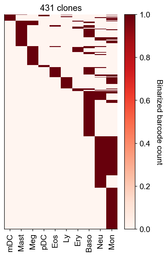
Show barcode heatmap as aggregated into given fate clusters (defined in adata_orig.obs['state_info'])

selected_times = None
selected_fates = [
    "Ccr7_DC",
    "Mast",
    "Meg",
    "pDC",
    "Eos",
    "Lymphoid",
    "Erythroid",
    "Baso",
    "Neutrophil",
    "Monocyte",
]
celltype_names = ["mDC", "Mast", "Meg", "pDC", "Eos", "Ly", "Ery", "Baso", "Neu", "Mon"]
cs.pl.barcode_heatmap(
    adata_orig,
    selected_times=selected_times,
    selected_fates=selected_fates,
    color_bar=True,
    rename_fates=celltype_names,
    log_transform=False,
    binarize=True,
)

Data saved at adata.uns['barcode_heatmap']

<Axes: title={'center': '431 clones'}>

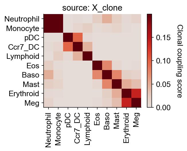
Fate coupling in the underlying clonal data, defined in our package as the normalized barcode covariance between cells annotated in different fates.

cs.tl.fate_coupling(
    adata_orig, selected_fates=selected_fates, source="X_clone"
)  # compute the fate coupling
cs.pl.fate_coupling(adata_orig, source="X_clone")  # actually plot the coupling

normalize by X_clone
each cluster do not have a unique time point. Simply column-normalize the matrix
Results saved as dictionary at adata.uns['fate_coupling_X_clone']

<Axes: title={'center': 'source: X_clone'}>

Fate hierarchy constructed from fate coupling of the underlying clonal data, using the neighbor-joining method.

cs.tl.fate_hierarchy(
    adata_orig, selected_fates=selected_fates, source="X_clone"
)  # compute the fate hierarchy
cs.pl.fate_hierarchy(adata_orig, source="X_clone")  # actually plot the hierarchy

normalize by X_clone
each cluster do not have a unique time point. Simply column-normalize the matrix
normalize by X_clone
each cluster do not have a unique time point. Simply column-normalize the matrix
normalize by X_clone
each cluster do not have a unique time point. Simply column-normalize the matrix
normalize by X_clone
each cluster do not have a unique time point. Simply column-normalize the matrix
normalize by X_clone
each cluster do not have a unique time point. Simply column-normalize the matrix
normalize by X_clone
each cluster do not have a unique time point. Simply column-normalize the matrix
normalize by X_clone
each cluster do not have a unique time point. Simply column-normalize the matrix
normalize by X_clone
each cluster do not have a unique time point. Simply column-normalize the matrix
Results saved as dictionary at adata.uns['fate_hierarchy_X_clone']

               /-Baso
            /-|
         /-|   \-Mast
        |  |
      /-|   \-Eos
     |  |
     |  |   /-Erythroid
   /-|   \-|
  |  |      \-Meg
  |  |
  |  |   /-Monocyte
--|   \-|
  |      \-Neutrophil
  |
  |      /-pDC
  |   /-|
   \-|   \-Ccr7_DC
     |
      \-Lymphoid

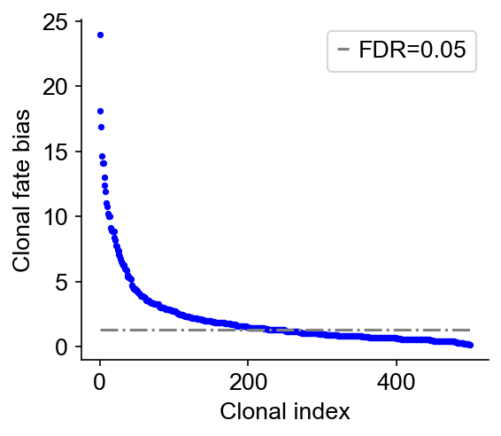
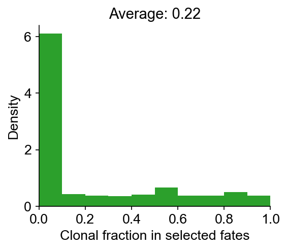
Next, we compute the clonal fate bias, -log(Q-value). We calculated a P-value that that a clone is enriched (or depleted) in a fate, using Fisher-Exact test (accounting for clone size). The P-value is then corrected to give a Q-value by Benjamini-Hochberg procedure. The alternative hypothesis options are: {‘two-sided’,‘greater’,‘less’}. The default is ‘two-sided’.

cs.tl.clonal_fate_bias(
    adata_orig, selected_fate="Monocyte", alternative="two-sided"
)  # compute the fate hierarchy
cs.pl.clonal_fate_bias(adata_orig)  # actually plot the hierarchy

100%|████████████████████████████████████████| 500/500 [00:00<00:00, 914.93it/s]

Data saved at adata.uns['clonal_fate_bias']

result = adata_orig.uns["clonal_fate_bias"]
result

	clone_id	clone_size	P_value	clonal_fraction_in_target_fate	Fate_bias
488	488	58	1.105140e-24	0.896552	23.956583
387	387	37	7.630927e-19	0.945946	18.117423
227	227	45	1.250056e-17	0.866667	16.903071
302	302	112	2.278106e-15	0.000000	14.642426
162	162	42	7.468800e-15	0.833333	14.126749
...	...	...	...	...	...
79	79	5	6.159379e-01	0.200000	0.210463
207	207	5	6.159379e-01	0.200000	0.210463
58	58	8	6.526613e-01	0.250000	0.185312
6	6	4	6.969634e-01	0.250000	0.156790
17	17	4	6.969634e-01	0.250000	0.156790

500 rows × 5 columns

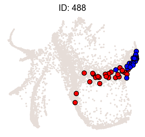
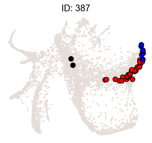
Illustrate some most biased clones.

ids = result["clone_id"][:2]
cs.pl.clones_on_manifold(
    adata_orig,
    selected_clone_list=ids,
    color_list=["black", "red", "blue"],
    clone_markersize=15,
)

ERROR: XMLRPC request failed [code: -32500]
RuntimeError: PyPI no longer supports 'pip search' (or XML-RPC search). Please use https://pypi.org/search (via a browser) instead. See https://warehouse.pypa.io/api-reference/xml-rpc.html#deprecated-methods for more information.