Hematopoiesis¶

Hematopoiesis dataset from Weinreb, C., Rodriguez-Fraticelli, A., Camargo, F. D. & Klein, A. M. Science 367, (2020).

This dataset has 3 time points for both the clonal and state measurements. It has ~50000 clonally-labeled cells. Running the whole pipeline for the first time could take 5.2 hours in a standard personal computer. Most of the time (3.3 h) is used for generating the similarity matrix, which are saved for later usage.

Key components:

Part I: Infer transition map from all clonal data
Part II: Infer transition using end-point clones
Part III: Infer transition map from state information alone
Part IV: Predict fate bias for Gata1+ states

[1]:

import cospar as cs
import numpy as np

[2]:

cs.logging.print_version()
cs.settings.verbosity = 2
cs.settings.data_path = "LARRY_data"  # A relative path to save data. If not existed before, create a new one.
cs.settings.figure_path = "LARRY_figure"  # A relative path to save figures. If not existed before, create a new one.
cs.settings.set_figure_params(
    format="png", figsize=[4, 3.5], dpi=75, fontsize=14, pointsize=2
)

Running cospar 0.2.0 (python 3.8.12) on 2022-02-07 21:21.

[3]:

# # This is for testing this notebook
# cs.settings.data_path='data_cospar'
# cs.settings.figure_path='fig_cospar'
# adata_orig=cs.datasets.hematopoiesis_subsampled()
# adata_orig.uns['data_des']=['LARRY_sp500_ranking1']

Loading data¶

[4]:

adata_orig = cs.datasets.hematopoiesis()

[5]:

adata_orig

[5]:

AnnData object with n_obs × n_vars = 49116 × 25289
    obs: 'time_info', 'state_info'
    uns: 'clonal_time_points', 'data_des', 'state_info_colors'
    obsm: 'X_clone', 'X_emb', 'X_pca'

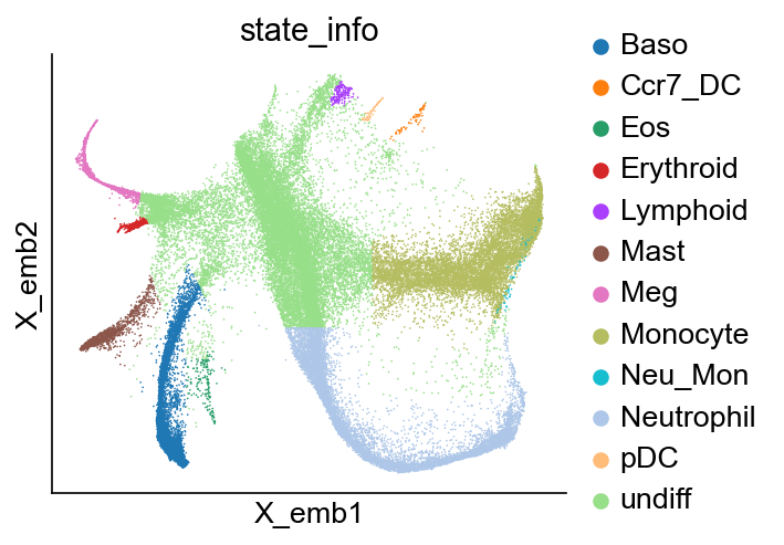
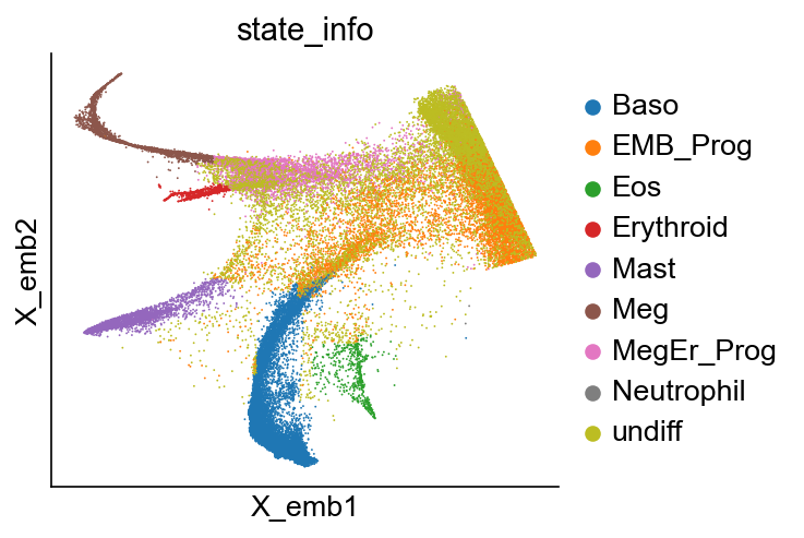
[6]:

cs.pl.embedding(adata_orig, color="state_info")

_images/20210121_all_hematopoietic_data_v3_8_0.png

[7]:

cs.hf.check_available_choices(adata_orig)

Available transition maps: []
Available clusters: ['undiff', 'Meg', 'Mast', 'Neu_Mon', 'Eos', 'Erythroid', 'Ccr7_DC', 'Baso', 'Lymphoid', 'pDC', 'Neutrophil', 'Monocyte']
Available time points: ['2' '4' '6']
Clonal time points: ['2' '4' '6']

Basic clonal analysis¶

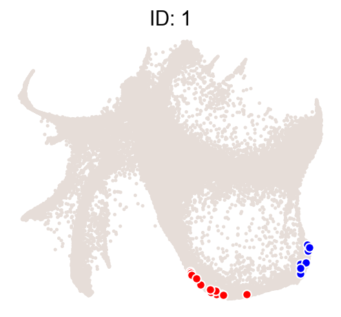
[8]:

cs.pl.clones_on_manifold(
    adata_orig, selected_clone_list=[1], color_list=["black", "red", "blue"]
)

_images/20210121_all_hematopoietic_data_v3_11_0.png

[9]:

selected_times = "4"
selected_fates = [
    "Ccr7_DC",
    "Mast",
    "Meg",
    "pDC",
    "Eos",
    "Lymphoid",
    "Erythroid",
    "Baso",
    "Neutrophil",
    "Monocyte",
]
cs.tl.fate_coupling(
    adata_orig,
    source="X_clone",
    selected_fates=selected_fates,
    selected_times=selected_times,
    normalize=False,
)
cs.pl.fate_coupling(adata_orig, source="X_clone")

Results saved as dictionary at adata.uns['fate_coupling_X_clone']

[9]:

<AxesSubplot:title={'center':'source: X_clone'}>

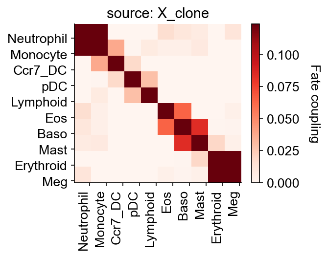
_images/20210121_all_hematopoietic_data_v3_12_2.png

[10]:

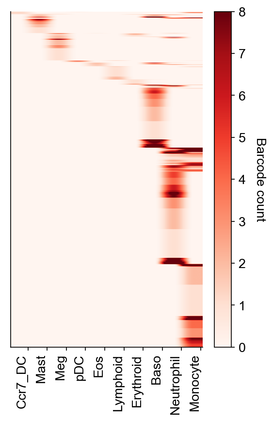
cs.pl.barcode_heatmap(
    adata_orig,
    selected_times=selected_times,
    selected_fates=selected_fates,
    color_bar=True,
)

Data saved at adata.uns['barcode_heatmap']

[10]:

<AxesSubplot:>

_images/20210121_all_hematopoietic_data_v3_13_2.png

Part I: Infer transition map from all clonal data¶

Map inference¶

When first run, it takes around 3 h 37 mins, in which 3 h 20 mins are used for computing the similarity matrices and saving these data. It takes only 20 mins for later runs.

[11]:

adata = cs.tmap.infer_Tmap_from_multitime_clones(
    adata_orig,
    clonal_time_points=["2", "4", "6"],
    later_time_point="6",
    smooth_array=[20, 15, 10],
    sparsity_threshold=0.2,
    max_iter_N=3,
)

Trying to set attribute `.uns` of view, copying.

------Compute the full Similarity matrix if necessary------
------Infer transition map between initial time points and the later time one------
--------Current initial time point: 2--------
Step 1: Select time points
Number of multi-time clones post selection: 1216
Step 2: Optimize the transition map recursively
Load pre-computed similarity matrix
Iteration 1, Use smooth_round=20
Iteration 2, Use smooth_round=15
Iteration 3, Use smooth_round=10
Convergence (CoSpar, iter_N=3): corr(previous_T, current_T)=0.903
--------Current initial time point: 4--------
Step 1: Select time points
Number of multi-time clones post selection: 3047
Step 2: Optimize the transition map recursively
Load pre-computed similarity matrix
Iteration 1, Use smooth_round=20
Iteration 2, Use smooth_round=15
Iteration 3, Use smooth_round=10
Convergence (CoSpar, iter_N=3): corr(previous_T, current_T)=0.97
-----------Total used time: 1604.8337297439575 s ------------

Save pre-computed data (optional)¶

[12]:

save_data = False
if save_data:
    cs.hf.save_map(adata)

Plotting¶

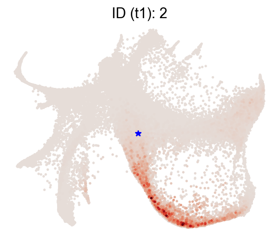
Transition profiles for single cells¶

Forward transitions with map_backward=False.

[13]:

selected_state_id_list = [2]

cs.pl.single_cell_transition(
    adata,
    selected_state_id_list=selected_state_id_list,
    color_bar=False,
    source="transition_map",
    map_backward=False,
)

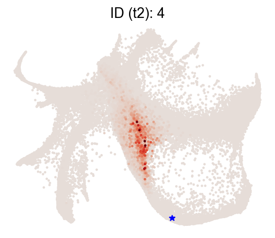
_images/20210121_all_hematopoietic_data_v3_22_0.png

Backward transitions with map_backward=True.

[14]:

selected_state_id_list = [4]
cs.pl.single_cell_transition(
    adata,
    selected_state_id_list=selected_state_id_list,
    color_bar=False,
    source="transition_map",
    map_backward=True,
)

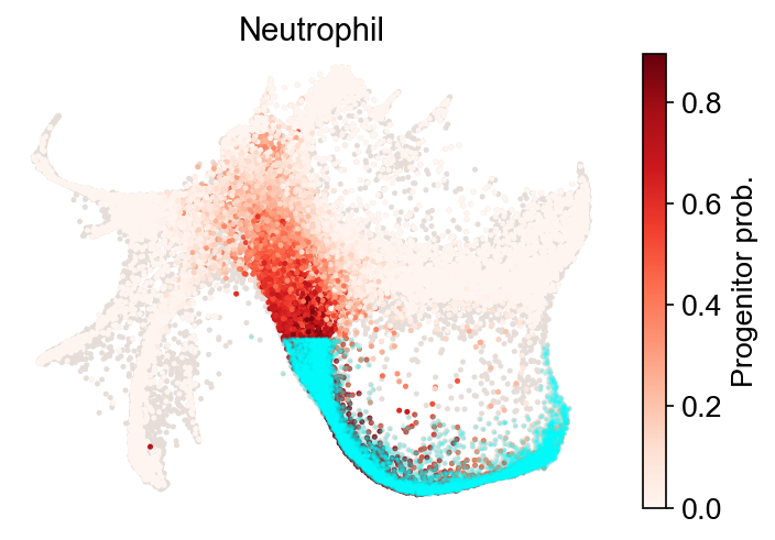
_images/20210121_all_hematopoietic_data_v3_24_0.png

Fate map¶

[15]:

cs.tl.fate_map(
    adata,
    selected_fates=["Neutrophil", "Monocyte"],
    source="transition_map",
    map_backward=True,
)
cs.pl.fate_map(
    adata,
    selected_fates=["Neutrophil"],
    source="transition_map",
    plot_target_state=True,
    show_histogram=False,
)

Results saved at adata.obs['fate_map_transition_map_Neutrophil']
Results saved at adata.obs['fate_map_transition_map_Monocyte']

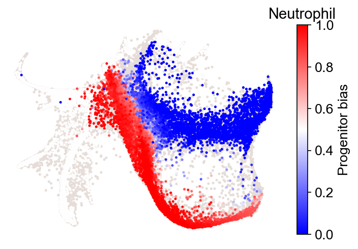
_images/20210121_all_hematopoietic_data_v3_26_1.png

Fate bias¶

[16]:

cs.tl.fate_bias(
    adata,
    selected_fates=["Neutrophil", "Monocyte"],
    source="transition_map",
    pseudo_count=0,
    sum_fate_prob_thresh=0.1,
)
cs.pl.fate_bias(
    adata,
    selected_fates=["Neutrophil", "Monocyte"],
    source="transition_map",
    plot_target_state=False,
    selected_times=["4"],
)

Results saved at adata.obs['fate_map_transition_map_Neutrophil']
Results saved at adata.obs['fate_map_transition_map_Monocyte']
Results saved at adata.obs['fate_bias_transition_map_Neutrophil*Monocyte']

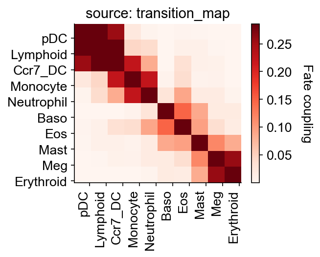
_images/20210121_all_hematopoietic_data_v3_28_1.png

Fate coupling from the transition map¶

[17]:

selected_fates = [
    "Ccr7_DC",
    "Mast",
    "Meg",
    "pDC",
    "Eos",
    "Lymphoid",
    "Erythroid",
    "Baso",
    "Neutrophil",
    "Monocyte",
]
cs.tl.fate_coupling(adata, selected_fates=selected_fates, source="transition_map")
cs.pl.fate_coupling(adata, source="transition_map")

Results saved as dictionary at adata.uns['fate_coupling_transition_map']

[17]:

<AxesSubplot:title={'center':'source: transition_map'}>

_images/20210121_all_hematopoietic_data_v3_30_2.png

Hierarchy¶

[18]:

cs.tl.fate_hierarchy(adata, selected_fates=selected_fates, source="transition_map")
cs.pl.fate_hierarchy(adata, source="transition_map")

Results saved as dictionary at adata.uns['fate_hierarchy_transition_map']

            /-Erythroid
         /-|
      /-|   \-Meg
     |  |
   /-|   \-Mast
  |  |
  |  |   /-Baso
  |   \-|
--|      \-Eos
  |
  |      /-Monocyte
  |   /-|
  |  |   \-Neutrophil
   \-|
     |      /-Lymphoid
     |   /-|
      \-|   \-Ccr7_DC
        |
         \-pDC

Dynamic trajectory inference¶

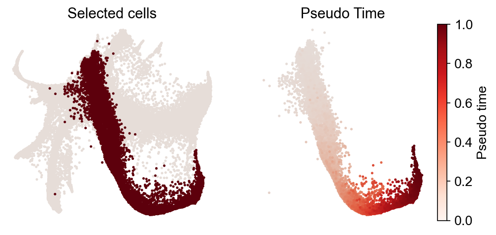
[19]:

cs.tl.progenitor(
    adata,
    selected_fates=["Neutrophil", "Monocyte"],
    source="transition_map",
    map_backward=True,
    bias_threshold_A=0.5,
    bias_threshold_B=0.5,
    sum_fate_prob_thresh=0.2,
    avoid_target_states=True,
)
cs.pl.progenitor(
    adata, selected_fates=["Neutrophil", "Monocyte"], source="transition_map"
)

Results saved at adata.obs['fate_map_transition_map_Neutrophil']
Results saved at adata.obs['fate_map_transition_map_Monocyte']
Results saved at adata.obs['fate_bias_transition_map_Neutrophil*Monocyte']
Results saved at adata.obs[f'progenitor_transition_map_Neutrophil'] and adata.obs[f'diff_trajectory_transition_map_Neutrophil']
Results saved at adata.obs[f'progenitor_transition_map_Monocyte'] and adata.obs[f'diff_trajectory_transition_map_Monocyte']

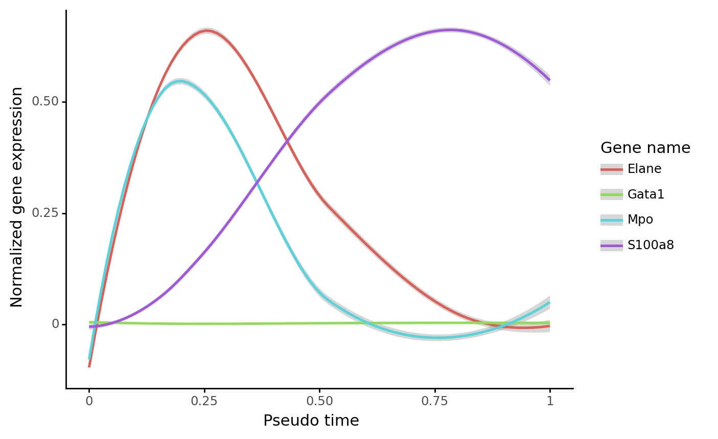
_images/20210121_all_hematopoietic_data_v3_34_1.png

_images/20210121_all_hematopoietic_data_v3_34_2.png

Gene trend along the dynamic trajectory¶

[20]:

gene_name_list = ["Gata1", "Mpo", "Elane", "S100a8"]
selected_fate = "Neutrophil"
cs.pl.gene_expression_dynamics(
    adata, selected_fate, gene_name_list, traj_threshold=0.2, invert_PseudoTime=False
)

_images/20210121_all_hematopoietic_data_v3_36_0.png

_images/20210121_all_hematopoietic_data_v3_36_1.png

Part II: Infer transition map from end-point clones¶

When run for the firs time, assuming that the similarity matrices are pre-computed, it takes 73 mins. Around 40 mins of which are used to compute the initialized map.

We group time points ‘2’ and ‘4’ so that the inference on day 2 states (which has much fewer cells) are better.

[21]:

time_info = np.array(adata_orig.obs["time_info"])
time_info[time_info == "2"] = "24"
time_info[time_info == "4"] = "24"
adata_orig.obs["time_info"] = time_info
adata_orig = cs.pp.initialize_adata_object(adata_orig)

Clones without any cells are removed.
Time points with clonal info: ['24' '6']
WARNING: Default ascending order of time points are: ['24' '6']. If not correct, run cs.hf.update_time_ordering for correction.
WARNING: Please make sure that the count matrix adata.X is NOT log-transformed.

[22]:

adata_1 = cs.tmap.infer_Tmap_from_one_time_clones(
    adata_orig,
    initial_time_points=["24"],
    later_time_point="6",
    initialize_method="OT",
    OT_cost="GED",
    smooth_array=[20, 15, 10],
    max_iter_N=[1, 3],
    sparsity_threshold=0.2,
    use_full_Smatrix=True,
)

Trying to set attribute `.uns` of view, copying.
Trying to set attribute `.uns` of view, copying.

--------Infer transition map between initial time points and the later time one-------
--------Current initial time point: 24--------
Step 0: Pre-processing and sub-sampling cells-------
Step 1: Use OT method for initialization-------
Load pre-computed custom OT matrix
Step 2: Jointly optimize the transition map and the initial clonal states-------
-----JointOpt Iteration 1: Infer initial clonal structure
-----JointOpt Iteration 1: Update the transition map by CoSpar
Load pre-computed similarity matrix
Iteration 1, Use smooth_round=20
Iteration 2, Use smooth_round=15
Iteration 3, Use smooth_round=10
Convergence (CoSpar, iter_N=3): corr(previous_T, current_T)=0.974
Convergence (JointOpt, iter_N=1): corr(previous_T, current_T)=0.144
Finishing Joint Optimization, used time 1308.7951350212097
-----------Total used time: 1341.8913249969482 s ------------

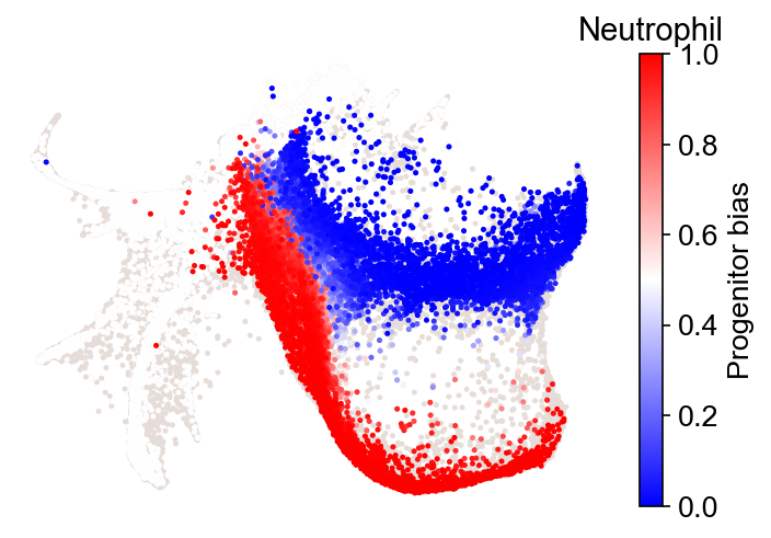
Fate bias¶

[23]:

cs.tl.fate_bias(
    adata_1,
    selected_fates=["Neutrophil", "Monocyte"],
    source="transition_map",
    pseudo_count=0,
    sum_fate_prob_thresh=0.1,
)
cs.pl.fate_bias(
    adata_1,
    selected_fates=["Neutrophil", "Monocyte"],
    source="transition_map",
    plot_target_state=False,
)

Results saved at adata.obs['fate_map_transition_map_Neutrophil']
Results saved at adata.obs['fate_map_transition_map_Monocyte']
Results saved at adata.obs['fate_bias_transition_map_Neutrophil*Monocyte']

_images/20210121_all_hematopoietic_data_v3_43_1.png

Part III: Infer transition map from state information alone¶

[24]:

adata_2 = cs.tmap.infer_Tmap_from_state_info_alone(
    adata_orig,
    initial_time_points=["24"],
    later_time_point="6",
    initialize_method="OT",
    OT_cost="GED",
    smooth_array=[20, 15, 10],
    max_iter_N=[1, 3],
    sparsity_threshold=0.2,
    use_full_Smatrix=True,
)

Step I: Generate pseudo clones where each cell has a unique barcode-----

Trying to set attribute `.uns` of view, copying.

Step II: Perform joint optimization-----

Trying to set attribute `.uns` of view, copying.

--------Infer transition map between initial time points and the later time one-------
--------Current initial time point: 24--------
Step 0: Pre-processing and sub-sampling cells-------
Step 1: Use OT method for initialization-------
Load pre-computed custom OT matrix
Step 2: Jointly optimize the transition map and the initial clonal states-------
-----JointOpt Iteration 1: Infer initial clonal structure
-----JointOpt Iteration 1: Update the transition map by CoSpar
Load pre-computed similarity matrix
Iteration 1, Use smooth_round=20
Iteration 2, Use smooth_round=15
Iteration 3, Use smooth_round=10
Convergence (CoSpar, iter_N=3): corr(previous_T, current_T)=0.977
Convergence (JointOpt, iter_N=1): corr(previous_T, current_T)=0.14
Finishing Joint Optimization, used time 1854.5912249088287
-----------Total used time: 1923.1848938465118 s ------------

[25]:

cs.tl.fate_bias(
    adata_2,
    selected_fates=["Neutrophil", "Monocyte"],
    source="transition_map",
    pseudo_count=0,
    sum_fate_prob_thresh=0.1,
)
cs.pl.fate_bias(
    adata_2,
    selected_fates=["Neutrophil", "Monocyte"],
    source="transition_map",
    plot_target_state=False,
)

Results saved at adata.obs['fate_map_transition_map_Neutrophil']
Results saved at adata.obs['fate_map_transition_map_Monocyte']
Results saved at adata.obs['fate_bias_transition_map_Neutrophil*Monocyte']

_images/20210121_all_hematopoietic_data_v3_46_1.png

Part IV: Predict fate bias for Gata1+ states¶

Load data¶

We load a dataset that also includes non-clonally labeled cells in the Gata1+ states (in total ~38K cells), which increases the statistical power of DGE analysis.

[26]:

cs.settings.data_path = "LARRY_data_Gata1"  # A relative path to save data. If not existed before, create a new one.
cs.settings.figure_path = "LARRY_figure_Gata1"  # A relative path to save figures. If not existed before, create a new one.
adata_orig_1 = cs.datasets.hematopoiesis_Gata1_states()

[27]:

adata_orig_1 = cs.pp.initialize_adata_object(adata_orig_1)

Time points with clonal info: ['2' '4' '6']
WARNING: Default ascending order of time points are: ['2' '4' '6']. If not correct, run cs.hf.update_time_ordering for correction.
WARNING: Please make sure that the count matrix adata.X is NOT log-transformed.

[28]:

cs.pl.embedding(adata_orig_1, color="time_info")

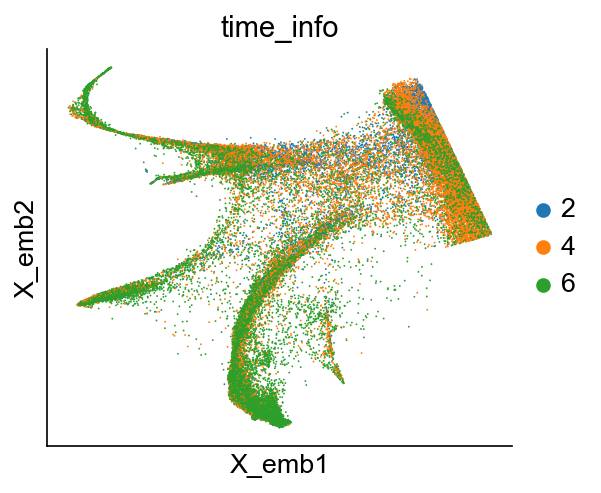
_images/20210121_all_hematopoietic_data_v3_52_0.png

[29]:

adata_orig_1

[29]:

AnnData object with n_obs × n_vars = 38457 × 25289
    obs: 'n_counts', 'Source', 'Well', 'mito_frac', 'time_info', 'state_info'
    var: 'highly_variable'
    uns: 'AllCellCyc_genes', 'clonal_time_points', 'data_des', 'max_mito', 'min_tot', 'new_highvar_genes', 'state_info_colors', 'time_info_colors', 'time_ordering'
    obsm: 'X_clone', 'X_emb', 'X_pca', 'X_umap'

[30]:

## This is for testing this notebook
# adata_orig_1=adata_orig
# adata_3=adata_1

Infer transition map from all clones¶

[31]:

adata_3 = cs.tmap.infer_Tmap_from_multitime_clones(
    adata_orig_1,
    later_time_point="6",
    smooth_array=[20, 15, 10],
    sparsity_threshold=0.1,
    intraclone_threshold=0.1,
    extend_Tmap_space=True,
)

------Compute the full Similarity matrix if necessary------

Trying to set attribute `.uns` of view, copying.

------Infer transition map between initial time points and the later time one------
--------Current initial time point: 2--------
Step 1: Select time points
Number of multi-time clones post selection: 355
Step 2: Optimize the transition map recursively
Load pre-computed similarity matrix
Iteration 1, Use smooth_round=20
Iteration 2, Use smooth_round=15
Iteration 3, Use smooth_round=10
Convergence (CoSpar, iter_N=3): corr(previous_T, current_T)=0.969
--------Current initial time point: 4--------
Step 1: Select time points
Number of multi-time clones post selection: 1270
Step 2: Optimize the transition map recursively
Load pre-computed similarity matrix
Iteration 1, Use smooth_round=20
Iteration 2, Use smooth_round=15
Iteration 3, Use smooth_round=10
Convergence (CoSpar, iter_N=3): corr(previous_T, current_T)=0.985
-----------Total used time: 477.8539500236511 s ------------

Fate bias¶

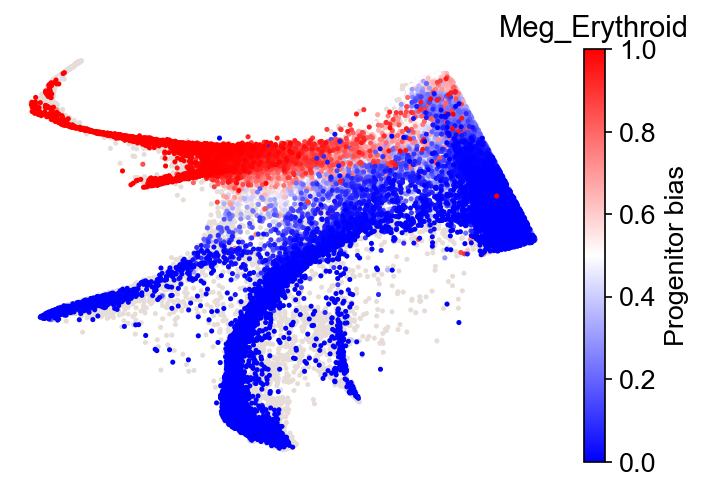
[32]:

selected_fates = [["Meg", "Erythroid"], ["Baso", "Mast", "Eos"]]
cs.tl.fate_bias(
    adata_3,
    selected_fates=selected_fates,
    source="transition_map",
    pseudo_count=0,
    sum_fate_prob_thresh=0.05,
)
cs.pl.fate_bias(
    adata_3,
    selected_fates=selected_fates,
    source="transition_map",
    plot_target_state=False,
)

Results saved at adata.obs['fate_map_transition_map_Meg_Erythroid']
Results saved at adata.obs['fate_map_transition_map_Baso_Mast_Eos']
Results saved at adata.obs['fate_bias_transition_map_Meg_Erythroid*Baso_Mast_Eos']

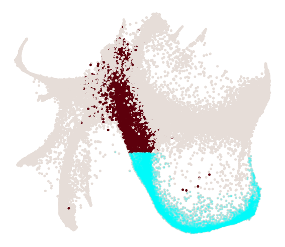
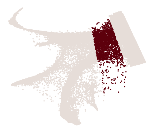
_images/20210121_all_hematopoietic_data_v3_58_1.png

Identify ancestor populations¶

[33]:

x_emb = adata_orig_1.obsm["X_emb"][:, 0]
y_emb = adata_orig_1.obsm["X_emb"][:, 1]

index_2 = cs.hf.above_the_line(adata_orig_1.obsm["X_emb"], [0, -500], [-300, 1000])
index_2_2 = cs.hf.above_the_line(adata_orig_1.obsm["X_emb"], [-450, -600], [-600, 800])

final_mask = (index_2_2) & (~index_2)  # & index_3 & index_4 & index_5 #mask_1 &
cs.pl.customized_embedding(x_emb, y_emb, final_mask)

[33]:

<AxesSubplot:>

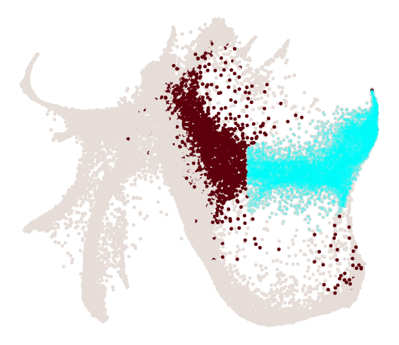
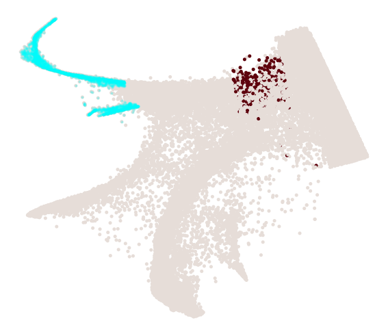
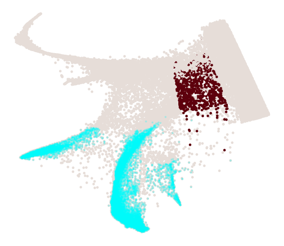
_images/20210121_all_hematopoietic_data_v3_60_1.png

[34]:

selected_fates = [["Meg", "Erythroid"], ["Baso", "Mast", "Eos"]]
cs.tl.progenitor(
    adata_3,
    selected_fates=selected_fates,
    source="transition_map",
    map_backward=True,
    bias_threshold_A=0.6,
    bias_threshold_B=0.3,
    sum_fate_prob_thresh=0.05,
    avoid_target_states=True,
)
cs.pl.progenitor(
    adata_3, selected_fates=selected_fates, source="transition_map", mask=final_mask
)

Results saved at adata.obs['fate_map_transition_map_Meg_Erythroid']
Results saved at adata.obs['fate_map_transition_map_Baso_Mast_Eos']
Results saved at adata.obs['fate_bias_transition_map_Meg_Erythroid*Baso_Mast_Eos']
Results saved at adata.obs[f'progenitor_transition_map_Meg_Erythroid'] and adata.obs[f'diff_trajectory_transition_map_Meg_Erythroid']
Results saved at adata.obs[f'progenitor_transition_map_Baso_Mast_Eos'] and adata.obs[f'diff_trajectory_transition_map_Baso_Mast_Eos']

_images/20210121_all_hematopoietic_data_v3_61_1.png

_images/20210121_all_hematopoietic_data_v3_61_2.png

DGE analysis¶

[35]:

cell_group_A = np.array(adata_3.obs[f"progenitor_transition_map_Meg_Erythroid"])
cell_group_B = np.array(adata_3.obs[f"progenitor_transition_map_Baso_Mast_Eos"])
dge_gene_A, dge_gene_B = cs.tl.differential_genes(
    adata_3, cell_group_A=cell_group_A, cell_group_B=cell_group_B, FDR_cutoff=0.05
)

[36]:

# All, ranked, DGE genes for group A
dge_gene_A

[36]:

	index	gene	Qvalue	mean_1	mean_2	ratio
0	4	Ctsg	0.000000e+00	0.103370	2.567811	-1.693123
1	3	Emb	0.000000e+00	0.186135	2.703714	-1.642705
2	26	Elane	3.264509e-241	0.151518	2.530409	-1.616299
3	2	Plac8	0.000000e+00	1.096986	4.811569	-1.470611
4	17	Igfbp4	0.000000e+00	1.042382	3.969988	-1.282990
...	...	...	...	...	...	...
965	2772	Rps29	2.823620e-02	2.905993	3.008932	-0.037529
966	2343	Rpl38	8.297305e-03	5.915980	6.061140	-0.029967
967	2976	Rpl5	4.697313e-02	4.714540	4.806636	-0.023065
968	2544	Ly6e	1.556172e-02	2.882883	2.944137	-0.022582
969	2705	Isg20	2.485104e-02	0.330973	0.342714	-0.012671

970 rows × 6 columns

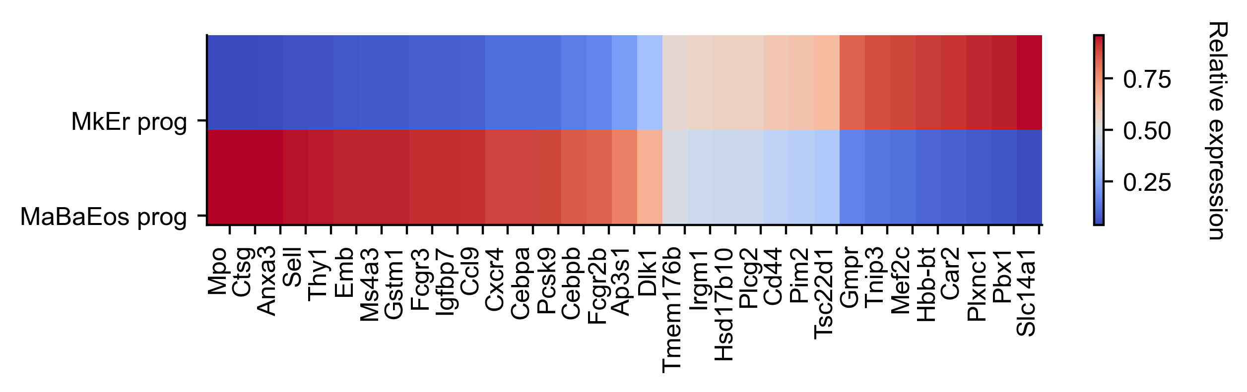
[37]:

sub_predicted_upper = [
    "Slc14a1",
    "Plxnc1",
    "Mef2c",
    "Tnip3",
    "Pbx1",
    "Hbb-bt",
    "Tmem176b",
    "Car2",
    "Pim2",
    "Tsc22d1",
    "Plcg2",
    "Gmpr",
    "Cd44",
    "Irgm1",
    "Hsd17b10",
    "Dlk1",
]
sub_predicted_lower = [
    "Ctsg",
    "Emb",
    "Ccl9",
    "Igfbp7",
    "Ap3s1",
    "Gstm1",
    "Ms4a3",
    "Fcgr3",
    "Mpo",
    "Cebpb",
    "Thy1",
    "Anxa3",
    "Sell",
    "Pcsk9",
    "Fcgr2b",
    "Cebpa",
    "Cxcr4",
]

[38]:

state_info = np.array(adata_3.obs["state_info"])
state_info[cell_group_A > 0] = "MegEr_Prog"
state_info[cell_group_B > 0] = "EMB_Prog"

[39]:

adata_3.obs["state_info"] = state_info
cs.pl.embedding(adata_3, color="state_info")

/Users/shouwenwang/miniconda3/envs/CoSpar_test/lib/python3.8/site-packages/anndata/_core/anndata.py:1220: FutureWarning: The `inplace` parameter in pandas.Categorical.reorder_categories is deprecated and will be removed in a future version. Reordering categories will always return a new Categorical object.
... storing 'state_info' as categorical

_images/20210121_all_hematopoietic_data_v3_67_1.png

[40]:

cs.settings.set_figure_params(
    format="pdf", figsize=[4, 3.5], dpi=200, fontsize=10, pointsize=3
)

gene_list = sub_predicted_upper + sub_predicted_lower
selected_fates = ["MegEr_Prog", "EMB_Prog"]
renames = ["MkEr prog", "MaBaEos prog"]

gene_expression_matrix = cs.pl.gene_expression_heatmap(
    adata_3,
    selected_genes=gene_list,
    selected_fates=selected_fates,
    rename_fates=renames,
    horizontal=True,
    fig_width=6.5,
    fig_height=2,
)

_images/20210121_all_hematopoietic_data_v3_68_0.png