Reprogramming
The reprogramming dataset from Biddy, B. A. et al. Nature 564, 219–224 (2018). This dataset has multiple time points for both clonal and state measurements.
Key components:
Part I: Infer transition map using clones from all time points
Part II: Infer transition map from end-point clones
Part III: Infer transition map from state information alone
Part IV: Predict early fate bias on day 3
[1]:
import cospar as cs
import numpy as np
[2]:
cs.logging.print_version()
cs.settings.verbosity = 2
cs.settings.set_figure_params(
    format="png", dpi=75, fontsize=14
)  # use png to reduce file size.

cs.settings.data_path = "CellTag_data"  # A relative path to save data. If not existed before, create a new one.
cs.settings.figure_path = "CellTag_figure"  # A relative path to save figures. If not existed before, create a new one.
Running cospar 0.2.0 (python 3.8.12) on 2022-02-07 22:21.
Loading data
[3]:
adata_orig = cs.datasets.reprogramming()
[4]:
adata_orig = cs.pp.initialize_adata_object(adata_orig)
Time points with clonal info: ['Day12' 'Day15' 'Day21' 'Day28' 'Day6' 'Day9']
WARNING: Default ascending order of time points are: ['Day12' 'Day15' 'Day21' 'Day28' 'Day6' 'Day9']. If not correct, run cs.hf.update_time_ordering for correction.
WARNING: Please make sure that the count matrix adata.X is NOT log-transformed.
[5]:
cs.hf.update_time_ordering(
    adata_orig, updated_ordering=["Day6", "Day9", "Day12", "Day15", "Day21", "Day28"]
)
The cells are barcoded over 3 rounds during the entire differentiation process. There are multiple ways to assemble the barcodes on day 0, day 3, and day 13 into a clonal ID. Below, we provide three variants:
Concatenate barcodes on day 0 and day 13, as in the original analysis (
adata_orig.obsm['X_clone_Concat_D0D3'], the default);Concatenate barcodes on day 0, day 3, and day 13 (
adata_orig.obsm['X_clone_Concat_D0D3D13']);No concatenation; each cell has up to 3 barcodes (
adata_orig.obsm['X_clone_NonConcat_D0D3D13']).
The last choice keeps the nested clonal structure in the data. You can choose any one of the clonal arrangement for downstream analysis, by setting adata_orig.obsm['X_clone']=adata_orig.obsm['X_clone_Concat_D0D3']. The three clonal arrangements give very similar fate prediction.
[6]:
adata_orig
[6]:
AnnData object with n_obs × n_vars = 18803 × 28001
    obs: 'time_info', 'state_info', 'reprogram_trajectory', 'failed_trajectory', 'Reference_fate_bias'
    uns: 'clonal_time_points', 'data_des', 'state_info_colors', 'time_info_colors', 'time_ordering'
    obsm: 'X_clone', 'X_clone_Concat_D0D3', 'X_clone_Concat_D0D3D13', 'X_clone_NonConcat_D0D3D13', 'X_emb', 'X_pca'
[7]:
cs.hf.check_available_choices(adata_orig)
Available transition maps: []
Available clusters: ['Reprogrammed', 'Failed', 'Others']
Available time points: ['Day6' 'Day9' 'Day12' 'Day15' 'Day21' 'Day28']
Clonal time points: ['Day6' 'Day9' 'Day12' 'Day15' 'Day21' 'Day28']
[8]:
re_propressing = False
if re_propressing:
cs.pp.get_highly_variable_genes(adata_orig)
cs.pp.remove_cell_cycle_correlated_genes(
adata_orig, corr_threshold=0.03, confirm_change=True
)
cs.pp.get_X_pca(adata_orig, n_pca_comp=40)
cs.pp.get_X_emb(adata_orig, n_neighbors=20, umap_min_dist=0.3)
# cs.pp.get_state_info(adata_orig,n_neighbors=20,resolution=0.5) # if this is changed, the cluster name used later will be wrong.
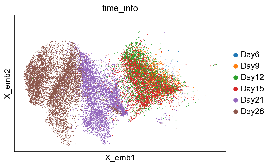
cs.pl.embedding(adata_orig, color="time_info")
[9]:
cs.pl.embedding(adata_orig, color="time_info")
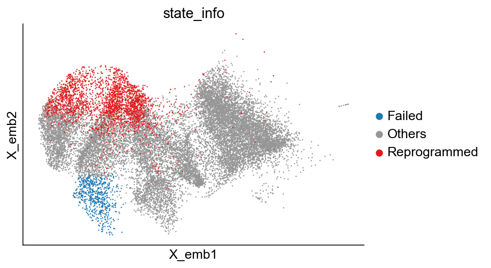
[10]:
cs.pl.embedding(adata_orig, color="state_info")
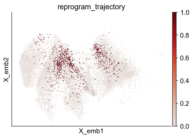
[11]:
adata_orig.obs["reprogram_trajectory"] = adata_orig.obs["reprogram_trajectory"].astype(
    int
)
cs.pl.embedding(adata_orig, color="reprogram_trajectory")
[12]:
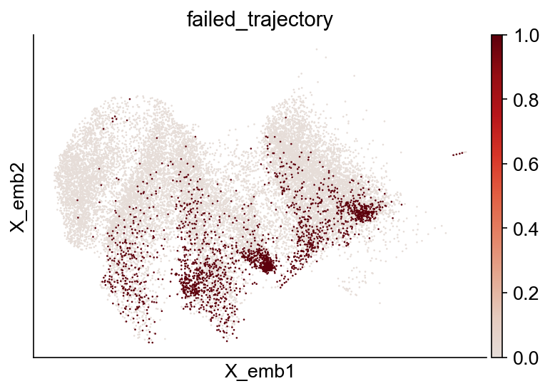
adata_orig.obs["failed_trajectory"] = adata_orig.obs["failed_trajectory"].astype(int)
cs.pl.embedding(adata_orig, color="failed_trajectory")
Basic clonal analysis
[13]:
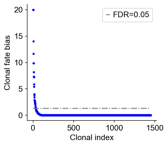
cs.tl.clonal_fate_bias(
    adata_orig, selected_fate="Reprogrammed", alternative="two-sided"
)
cs.pl.clonal_fate_bias(adata_orig)
100%|██████████| 1451/1451 [00:01<00:00, 792.99it/s]
Data saved at adata.uns['clonal_fate_bias']

[14]:
result = adata_orig.uns["clonal_fate_bias"]
result
[14]:
| Clone_ID | Clone_size | Q_value | Fate_bias | clonal_fraction_in_target_fate | |
|---|---|---|---|---|---|
| 0 | 1014 | 2382.0 | 1.000000e-20 | 20.000000 | 0.371537 |
| 1 | 611 | 1908.0 | 1.000000e-20 | 20.000000 | 0.265199 |
| 2 | 600 | 780.0 | 1.000000e-20 | 20.000000 | 0.014103 |
| 3 | 1188 | 289.0 | 1.000000e-20 | 20.000000 | 0.446367 |
| 4 | 545 | 283.0 | 9.769878e-15 | 14.010111 | 0.007067 |
| ... | ... | ... | ... | ... | ... |
| 1446 | 497 | 4.0 | 1.000000e+00 | -0.000000 | 0.000000 |
| 1447 | 496 | 1.0 | 1.000000e+00 | -0.000000 | 1.000000 |
| 1448 | 494 | 22.0 | 1.000000e+00 | -0.000000 | 0.227273 |
| 1449 | 504 | 1.0 | 1.000000e+00 | -0.000000 | 0.000000 |
| 1450 | 1450 | 3.0 | 1.000000e+00 | -0.000000 | 0.000000 |
1451 rows × 5 columns
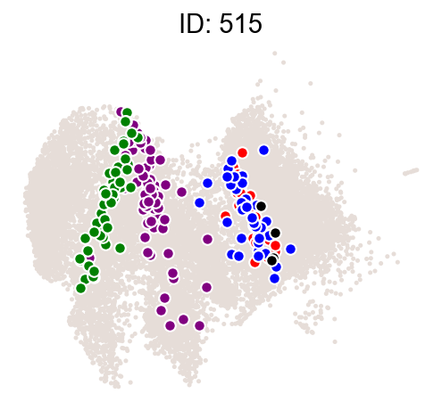
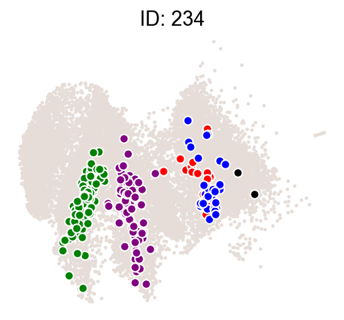
[15]:
ids = result["clone_id"][8:10]
# ids=[324,313,446,716,367]
cs.pl.clones_on_manifold(adata_orig, selected_clone_list=ids)
Part I: Infer transition map using clones from all time points
Map inference
Running it the first time takes ~20 mins, ~17 mins of which are used to compute the similarity matrix. When it is run again, it only takes ~3 mins.
[16]:
adata = cs.tmap.infer_Tmap_from_multitime_clones(
    adata_orig,
    clonal_time_points=["Day15", "Day21"],
    later_time_point="Day28",
    smooth_array=[15, 10, 5],
    sparsity_threshold=0.2,
    intraclone_threshold=0.2,
)
Trying to set attribute `.uns` of view, copying.
------Compute the full Similarity matrix if necessary------
------Infer transition map between initial time points and the later time one------
--------Current initial time point: Day15--------
Step 1: Select time points
Number of multi-time clones post selection: 179
Step 2: Optimize the transition map recursively
Load pre-computed similarity matrix
Iteration 1, Use smooth_round=15
Iteration 2, Use smooth_round=10
Iteration 3, Use smooth_round=5
Convergence (CoSpar, iter_N=3): corr(previous_T, current_T)=0.929
Iteration 4, Use smooth_round=5
Convergence (CoSpar, iter_N=4): corr(previous_T, current_T)=0.995
--------Current initial time point: Day21--------
Step 1: Select time points
Number of multi-time clones post selection: 226
Step 2: Optimize the transition map recursively
Load pre-computed similarity matrix
Iteration 1, Use smooth_round=15
Iteration 2, Use smooth_round=10
Iteration 3, Use smooth_round=5
Convergence (CoSpar, iter_N=3): corr(previous_T, current_T)=0.921
Iteration 4, Use smooth_round=5
Convergence (CoSpar, iter_N=4): corr(previous_T, current_T)=0.99
-----------Total used time: 165.4444100856781 s ------------
[17]:
cs.hf.check_available_map(adata)
adata.uns["available_map"]
[17]:
['transition_map', 'intraclone_transition_map']
Save or load pre-computed data
This can be used to save adata with maps computed from different tools or parameters. Usually, different parameter choices will result in different data_des, a prefix to identify the anndata. Saving an adata would print the data_des, which can be used to load the corresponding adata.
[18]:
save_data = False
if save_data:
    cs.hf.save_map(adata)

load_data = False
if load_data:
    # file_path='CellTag_data/cospar_MultiTimeClone_Later_FullSpace0_t*Day15*Day21*Day28_adata_with_transition_map.h5ad'
    adata = cs.hf.read(file_path)
[19]:
cs.hf.check_available_choices(adata)
WARNING: Pre-computed time_ordering does not include the right time points. Re-compute it!
Available transition maps: ['transition_map', 'intraclone_transition_map']
Available clusters: ['Reprogrammed', 'Failed', 'Others']
Available time points: ['Day15' 'Day21' 'Day28']
Clonal time points: ['Day15' 'Day21' 'Day28']
Plotting
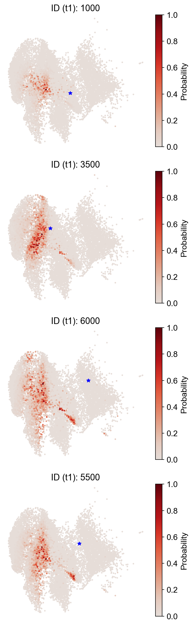
Single-cell transitions
[20]:
selected_state_id_list = [1000, 3500, 6000, 5500]

cs.pl.single_cell_transition(
    adata,
    selected_state_id_list=selected_state_id_list,
    source="transition_map",
    map_backward=False,
)
Fate map
[21]:
cs.tl.fate_map(
    adata,
    selected_fates=["Reprogrammed", "Failed"],
    source="transition_map",
    map_backward=True,
)
cs.pl.fate_map(
    adata,
    selected_fates=["Reprogrammed", "Failed"],
    source="transition_map",
    plot_target_state=True,
)
Results saved at adata.obs['fate_map_transition_map_Reprogrammed']
Results saved at adata.obs['fate_map_transition_map_Failed']
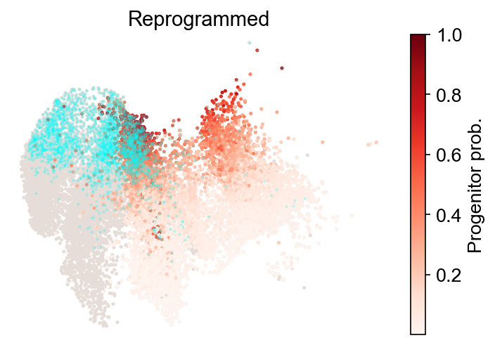
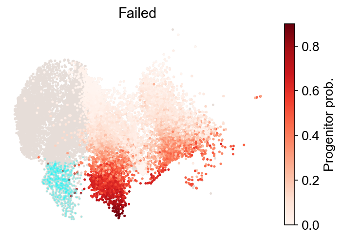
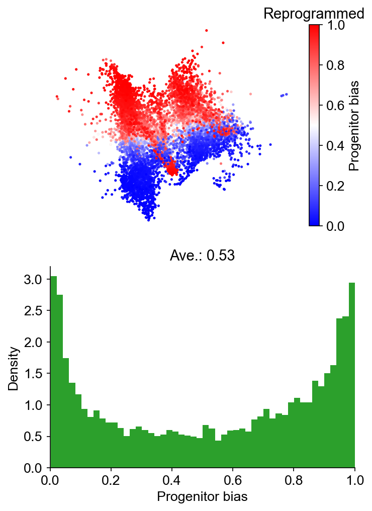
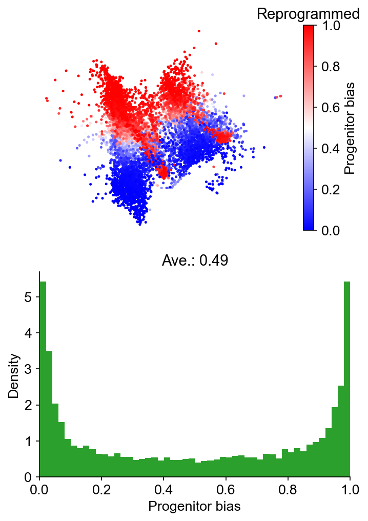
Fate bias
[22]:
cs.tl.fate_bias(
    adata,
    selected_fates=["Reprogrammed", "Failed"],
    source="transition_map",
    map_backward=True,
    method="norm-sum",
)
cs.pl.fate_bias(
    adata,
    selected_fates=["Reprogrammed", "Failed"],
    source="transition_map",
    plot_target_state=False,
    background=False,
    show_histogram=True,
)
Results saved at adata.obs['fate_map_transition_map_Reprogrammed']
Results saved at adata.obs['fate_map_transition_map_Failed']
Results saved at adata.obs['fate_bias_transition_map_Reprogrammed*Failed']
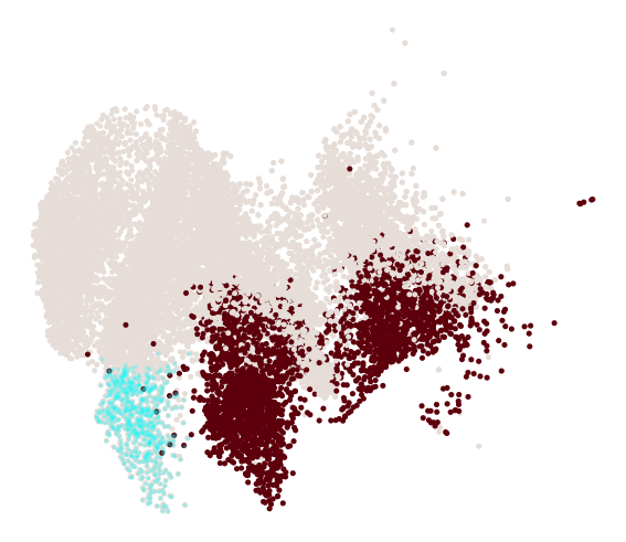
Identify differentially expressed genes
[23]:
selected_fates = ["Reprogrammed", "Failed"]
cs.tl.progenitor(
    adata,
    selected_fates,
    source="transition_map",
    sum_fate_prob_thresh=0.2,
    bias_threshold_A=0.5,
    bias_threshold_B=0.5,
)
cs.pl.progenitor(adata, selected_fates, source="transition_map")
Results saved at adata.obs['fate_map_transition_map_Reprogrammed']
Results saved at adata.obs['fate_map_transition_map_Failed']
Results saved at adata.obs['fate_bias_transition_map_Reprogrammed*Failed']
Results saved at adata.obs[f'progenitor_transition_map_Reprogrammed'] and adata.obs[f'diff_trajectory_transition_map_Reprogrammed']
Results saved at adata.obs[f'progenitor_transition_map_Failed'] and adata.obs[f'diff_trajectory_transition_map_Failed']
Differential genes for two ancestor groups
[24]:
cell_group_A = np.array(adata.obs[f"progenitor_transition_map_Reprogrammed"])
cell_group_B = np.array(adata.obs[f"progenitor_transition_map_Failed"])
dge_gene_A, dge_gene_B = cs.tl.differential_genes(
    adata, cell_group_A=cell_group_A, cell_group_B=cell_group_B, FDR_cutoff=0.05
)
[25]:
# All, ranked, DGE genes for group A
dge_gene_A
[25]:
| index | gene | Qvalue | mean_1 | mean_2 | ratio | |
|---|---|---|---|---|---|---|
| 0 | 35 | Col3a1 | 6.087368e-223 | 0.807060 | 5.999794 | -1.953668 |
| 1 | 57 | Col1a2 | 1.345045e-161 | 0.297653 | 3.076256 | -1.651340 |
| 2 | 41 | Spp1 | 3.197045e-207 | 10.833703 | 32.003143 | -1.479702 |
| 3 | 9 | Col1a1 | 0.000000e+00 | 2.036317 | 7.257215 | -1.443333 |
| 4 | 6 | Il6st | 0.000000e+00 | 2.108766 | 7.134142 | -1.387648 |
| ... | ... | ... | ... | ... | ... | ... |
| 4828 | 5607 | Tbk1 | 2.006752e-02 | 0.224493 | 0.224873 | -0.000448 |
| 4829 | 5172 | Sec23a | 1.005175e-02 | 0.344517 | 0.344837 | -0.000344 |
| 4830 | 6047 | Ints5 | 3.603720e-02 | 0.226673 | 0.226857 | -0.000216 |
| 4831 | 5737 | Taf2 | 2.431736e-02 | 0.278397 | 0.278525 | -0.000144 |
| 4832 | 6101 | Dgkq | 3.874214e-02 | 0.144835 | 0.144836 | -0.000002 |
4833 rows × 6 columns
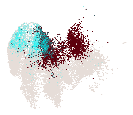
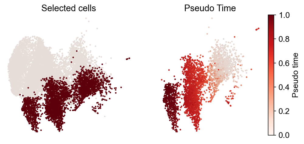
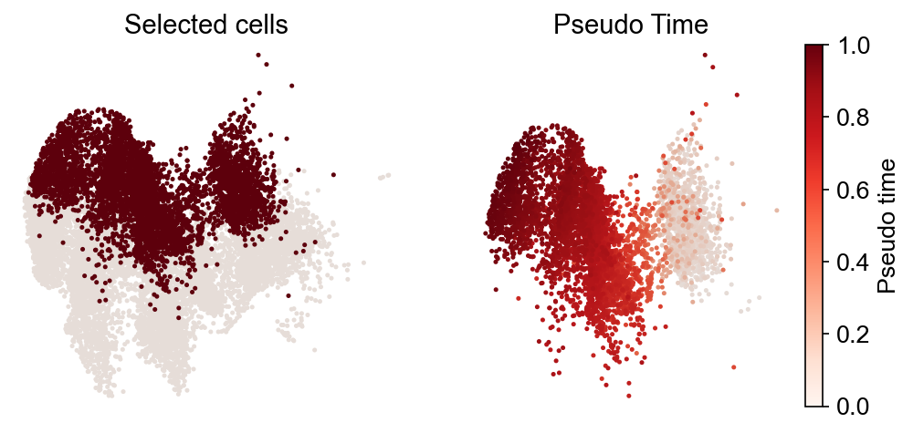
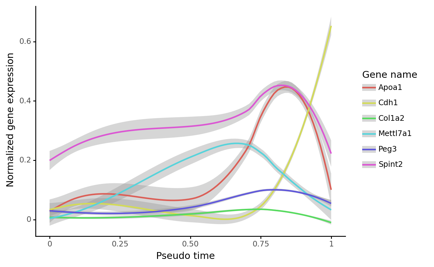
Gene trend along the trajectory
The results are based on pre-computed dynamic trajectories from the preceding step. It is better to use the intraclone_transition_map. First, show the expression dynamics along the failed trajectory:
[26]:
gene_name_list = ["Col1a2", "Apoa1", "Peg3", "Spint2", "Mettl7a1", "Cdh1"]
selected_fate = "Failed"
cs.pl.gene_expression_dynamics(
    adata, selected_fate, gene_name_list, traj_threshold=0.1, invert_PseudoTime=True
)
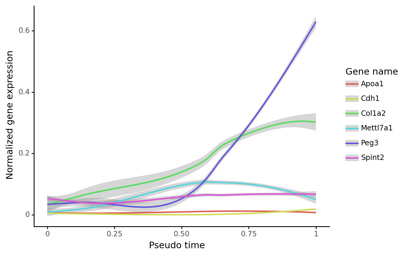
Expression dynamics along the reprogramming trajectory:
[27]:
gene_name_list = ["Col1a2", "Apoa1", "Peg3", "Spint2", "Mettl7a1", "Cdh1"]
selected_fate = "Reprogrammed"
cs.pl.gene_expression_dynamics(
    adata, selected_fate, gene_name_list, traj_threshold=0.1, invert_PseudoTime=True
)
Part II: Infer transition map from end-point clones¶¶
It takes ~12 mins to compute for the first time (excluding the time for computing similarity matrix); and ~5 mins later.
[28]:
adata = cs.tmap.infer_Tmap_from_one_time_clones(
    adata_orig,
    initial_time_points=["Day15", "Day21"],
    later_time_point="Day28",
    initialize_method="OT",
    OT_cost="SPD",
    smooth_array=[15, 10, 5],
    sparsity_threshold=0.2,
)
Trying to set attribute `.uns` of view, copying.
Trying to set attribute `.uns` of view, copying.
--------Infer transition map between initial time points and the later time one-------
--------Current initial time point: Day15--------
Step 0: Pre-processing and sub-sampling cells-------
Step 1: Use OT method for initialization-------
Load pre-computed shortest path distance matrix
Compute new custom OT matrix
Use uniform growth rate
OT solver: duality_gap
Finishing computing optial transport map, used time 51.17336821556091
Step 2: Jointly optimize the transition map and the initial clonal states-------
-----JointOpt Iteration 1: Infer initial clonal structure
-----JointOpt Iteration 1: Update the transition map by CoSpar
Load pre-computed similarity matrix
Iteration 1, Use smooth_round=15
Iteration 2, Use smooth_round=10
Iteration 3, Use smooth_round=5
Convergence (CoSpar, iter_N=3): corr(previous_T, current_T)=0.875
Iteration 4, Use smooth_round=5
Convergence (CoSpar, iter_N=4): corr(previous_T, current_T)=0.992
Convergence (JointOpt, iter_N=1): corr(previous_T, current_T)=0.276
Finishing Joint Optimization, used time 80.46711325645447
Trying to set attribute `.uns` of view, copying.
--------Current initial time point: Day21--------
Step 0: Pre-processing and sub-sampling cells-------
Step 1: Use OT method for initialization-------
Load pre-computed shortest path distance matrix
Compute new custom OT matrix
Use uniform growth rate
OT solver: duality_gap
Finishing computing optial transport map, used time 98.62810587882996
Step 2: Jointly optimize the transition map and the initial clonal states-------
-----JointOpt Iteration 1: Infer initial clonal structure
-----JointOpt Iteration 1: Update the transition map by CoSpar
Load pre-computed similarity matrix
Iteration 1, Use smooth_round=15
Iteration 2, Use smooth_round=10
Iteration 3, Use smooth_round=5
Convergence (CoSpar, iter_N=3): corr(previous_T, current_T)=0.896
Iteration 4, Use smooth_round=5
Convergence (CoSpar, iter_N=4): corr(previous_T, current_T)=0.987
Convergence (JointOpt, iter_N=1): corr(previous_T, current_T)=0.15
Finishing Joint Optimization, used time 162.67132997512817
-----------Total used time: 408.8195090293884 s ------------
[29]:
cs.hf.check_available_map(adata)
adata.uns["available_map"]
[29]:
['transition_map', 'OT_transition_map']
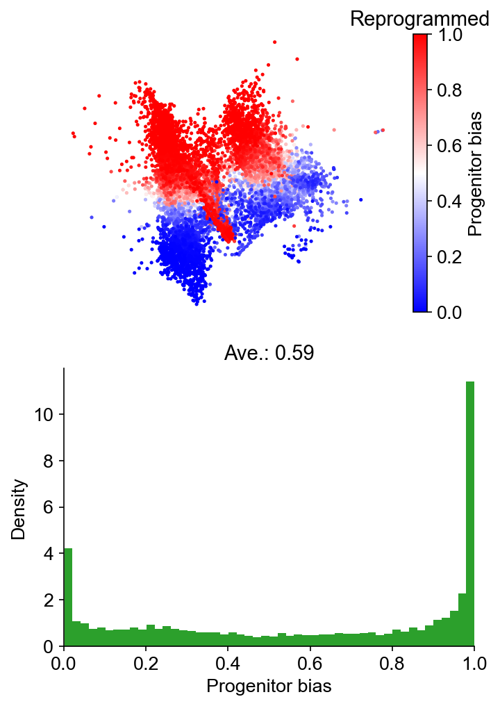
Fate bias
[30]:
cs.tl.fate_bias(
    adata,
    selected_fates=["Reprogrammed", "Failed"],
    source="transition_map",
    map_backward=True,
    method="norm-sum",
)
cs.pl.fate_bias(
    adata,
    selected_fates=["Reprogrammed", "Failed"],
    source="transition_map",
    plot_target_state=False,
    background=False,
    show_histogram=True,
)
Results saved at adata.obs['fate_map_transition_map_Reprogrammed']
Results saved at adata.obs['fate_map_transition_map_Failed']
Results saved at adata.obs['fate_bias_transition_map_Reprogrammed*Failed']
Part III: Infer transition map from state information alone
It takes ~5 mins
[31]:
adata = cs.tmap.infer_Tmap_from_state_info_alone(
    adata_orig,
    initial_time_points=["Day15", "Day21"],
    later_time_point="Day28",
    initialize_method="OT",
    OT_cost="SPD",
    smooth_array=[15, 10, 5],
    sparsity_threshold=0.2,
    use_full_Smatrix=True,
)
Step I: Generate pseudo clones where each cell has a unique barcode-----
Trying to set attribute `.uns` of view, copying.
Step II: Perform joint optimization-----
Trying to set attribute `.uns` of view, copying.
--------Infer transition map between initial time points and the later time one-------
--------Current initial time point: Day15--------
Step 0: Pre-processing and sub-sampling cells-------
Step 1: Use OT method for initialization-------
Load pre-computed shortest path distance matrix
Compute new custom OT matrix
Use uniform growth rate
OT solver: duality_gap
Finishing computing optial transport map, used time 42.353046894073486
Step 2: Jointly optimize the transition map and the initial clonal states-------
-----JointOpt Iteration 1: Infer initial clonal structure
-----JointOpt Iteration 1: Update the transition map by CoSpar
Load pre-computed similarity matrix
Iteration 1, Use smooth_round=15
Iteration 2, Use smooth_round=10
Iteration 3, Use smooth_round=5
Convergence (CoSpar, iter_N=3): corr(previous_T, current_T)=0.877
Iteration 4, Use smooth_round=5
Convergence (CoSpar, iter_N=4): corr(previous_T, current_T)=0.994
Convergence (JointOpt, iter_N=1): corr(previous_T, current_T)=0.301
Finishing Joint Optimization, used time 97.98227381706238
Trying to set attribute `.uns` of view, copying.
--------Current initial time point: Day21--------
Step 0: Pre-processing and sub-sampling cells-------
Step 1: Use OT method for initialization-------
Load pre-computed shortest path distance matrix
Compute new custom OT matrix
Use uniform growth rate
OT solver: duality_gap
Finishing computing optial transport map, used time 125.77742171287537
Step 2: Jointly optimize the transition map and the initial clonal states-------
-----JointOpt Iteration 1: Infer initial clonal structure
-----JointOpt Iteration 1: Update the transition map by CoSpar
Load pre-computed similarity matrix
Iteration 1, Use smooth_round=15
Iteration 2, Use smooth_round=10
Iteration 3, Use smooth_round=5
Convergence (CoSpar, iter_N=3): corr(previous_T, current_T)=0.897
Iteration 4, Use smooth_round=5
Convergence (CoSpar, iter_N=4): corr(previous_T, current_T)=0.984
Convergence (JointOpt, iter_N=1): corr(previous_T, current_T)=0.29
Finishing Joint Optimization, used time 114.50927495956421
-----------Total used time: 393.1687672138214 s ------------
[32]:
cs.hf.check_available_map(adata)
adata.uns["available_map"]
[32]:
['transition_map', 'OT_transition_map']
Fate bias
[33]:
cs.tl.fate_bias(
    adata,
    selected_fates=["Reprogrammed", "Failed"],
    source="transition_map",
    map_backward=True,
    method="norm-sum",
)
cs.pl.fate_bias(
    adata,
    selected_fates=["Reprogrammed", "Failed"],
    source="transition_map",
    plot_target_state=False,
    background=False,
    show_histogram=True,
)
Results saved at adata.obs['fate_map_transition_map_Reprogrammed']
Results saved at adata.obs['fate_map_transition_map_Failed']
Results saved at adata.obs['fate_bias_transition_map_Reprogrammed*Failed']
Part IV: Predict early fate bias on day 3
Load data
The above dataset only includes clonally-labeled states from day 6 to day 28. We load a dataset that has day-0 and day-3 states, which do not have clonal information.
[34]:
cs.settings.data_path = "CellTag_data_full"  # A relative path to save data. If not existed before, create a new one.
cs.settings.figure_path = "CellTag_figure_full"  # A relative path to save figures. If not existed before, create a new one.
adata_orig_1 = cs.datasets.reprogramming_Day0_3_28()
[35]:
adata_orig_1 = cs.pp.initialize_adata_object(adata_orig_1)
Time points with clonal info: ['Day28']
WARNING: Default ascending order of time points are: ['Day0' 'Day28' 'Day3']. If not correct, run cs.hf.update_time_ordering for correction.
WARNING: Please make sure that the count matrix adata.X is NOT log-transformed.
[36]:
cs.hf.update_time_ordering(adata_orig_1, updated_ordering=["Day0", "Day3", "Day28"])
[37]:
cs.pl.embedding(adata_orig_1, color="time_info")
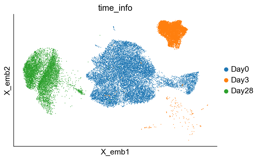
[38]:
adata_orig_1
[38]:
AnnData object with n_obs × n_vars = 27718 × 28001
    obs: 'predicted_doublet', 'row_counts', 'time_info', 'state_info', 'batch'
    var: 'highly_variable-0'
    uns: 'clonal_time_points', 'data_des', 'state_info_colors', 'time_info_colors', 'time_ordering'
    obsm: 'X_clone', 'X_emb', 'X_emb_old', 'X_emb_v1', 'X_pca'
Infer transition map from end-point clones¶¶
It takes ~4 mins
[39]:
adata_1 = cs.tmap.infer_Tmap_from_one_time_clones(
    adata_orig_1,
    initial_time_points=["Day3"],
    later_time_point=["Day28"],
    initialize_method="HighVar",
    smooth_array=[15, 10, 5],
    max_iter_N=[1, 3],
    sparsity_threshold=0.2,
    use_full_Smatrix=True,
)
Trying to set attribute `.uns` of view, copying.
Trying to set attribute `.uns` of view, copying.
--------Infer transition map between initial time points and the later time one-------
--------Current initial time point: Day3--------
Step 0: Pre-processing and sub-sampling cells-------
Step 1: Use the HighVar method for initialization-------
Step a: find the commonly shared highly variable genes------
Highly varable gene number: 1684 (t1); 1696 (t2). Common set: 960
Step b: convert the shared highly variable genes into clonal info------
92%|█████████▎| 888/960 [00:00<00:00, 1292.96it/s]
Total used genes=888 (no cells left)
Step c: compute the transition map based on clonal info from highly variable genes------
Load pre-computed similarity matrix
Iteration 1, Use smooth_round=15
Iteration 2, Use smooth_round=10
Iteration 3, Use smooth_round=5
Convergence (CoSpar, iter_N=3): corr(previous_T, current_T)=0.862
Finishing initialization using HighVar, used time 158.03640127182007
Step 2: Jointly optimize the transition map and the initial clonal states-------
-----JointOpt Iteration 1: Infer initial clonal structure
-----JointOpt Iteration 1: Update the transition map by CoSpar
Load pre-computed similarity matrix
Iteration 1, Use smooth_round=15
Iteration 2, Use smooth_round=10
Iteration 3, Use smooth_round=5
Convergence (CoSpar, iter_N=3): corr(previous_T, current_T)=0.921
Convergence (JointOpt, iter_N=1): corr(previous_T, current_T)=0.512
Finishing Joint Optimization, used time 126.52328705787659
-----------Total used time: 289.5595648288727 s ------------
Fate bias
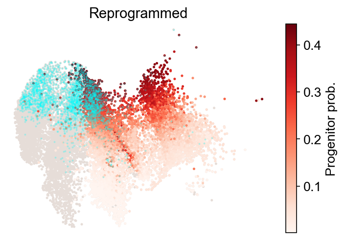
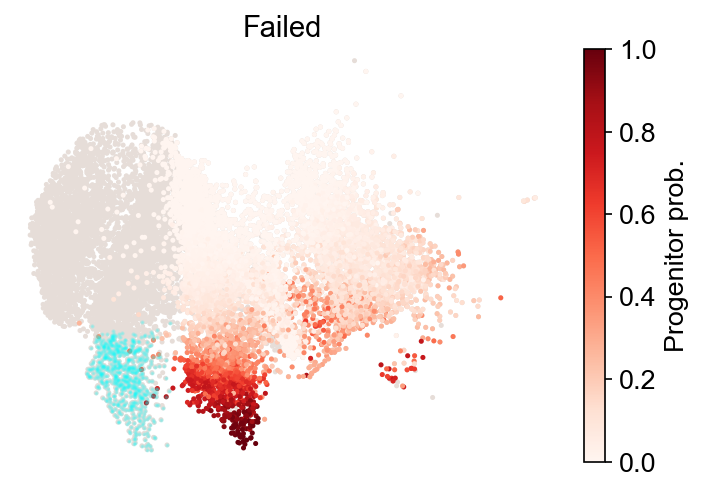
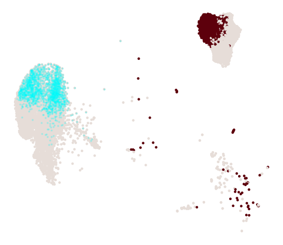
[40]:
cs.tl.fate_map(
    adata,
    selected_fates=["Reprogrammed", "Failed"],
    source="transition_map",
    map_backward=True,
)
cs.pl.fate_map(
    adata,
    selected_fates=["Reprogrammed", "Failed"],
    source="transition_map",
    plot_target_state=True,
)
Use pre-computed fate map
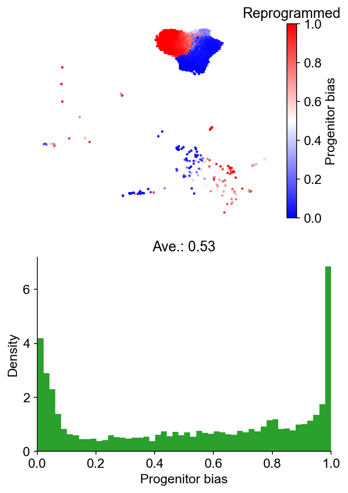
[41]:
cs.tl.fate_bias(
    adata_1,
    selected_fates=["Reprogrammed", "Failed"],
    source="transition_map",
    map_backward=True,
    method="norm-sum",
)
cs.pl.fate_bias(
    adata_1,
    selected_fates=["Reprogrammed", "Failed"],
    source="transition_map",
    selected_times=["Day3"],
    plot_target_state=False,
    background=False,
    show_histogram=True,
)
Results saved at adata.obs['fate_map_transition_map_Reprogrammed']
Results saved at adata.obs['fate_map_transition_map_Failed']
Results saved at adata.obs['fate_bias_transition_map_Reprogrammed*Failed']
Identify ancestor populations
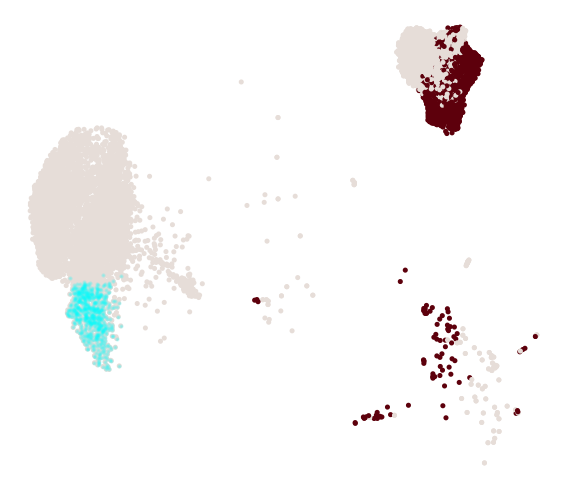
[42]:
selected_fates = ["Reprogrammed", "Failed"]
cs.tl.progenitor(
    adata_1,
    selected_fates,
    source="transition_map",
    sum_fate_prob_thresh=0.1,
    bias_threshold_A=0.5,
    bias_threshold_B=0.5,
)
cs.pl.progenitor(adata_1, selected_fates, source="transition_map")
Results saved at adata.obs['fate_map_transition_map_Reprogrammed']
Results saved at adata.obs['fate_map_transition_map_Failed']
Results saved at adata.obs['fate_bias_transition_map_Reprogrammed*Failed']
Results saved at adata.obs[f'progenitor_transition_map_Reprogrammed'] and adata.obs[f'diff_trajectory_transition_map_Reprogrammed']
Results saved at adata.obs[f'progenitor_transition_map_Failed'] and adata.obs[f'diff_trajectory_transition_map_Failed']
DGE analysis
[43]:
cell_group_A = np.array(adata_1.obs[f"progenitor_transition_map_Reprogrammed"])
cell_group_B = np.array(adata_1.obs[f"progenitor_transition_map_Failed"])
dge_gene_A, dge_gene_B = cs.tl.differential_genes(
    adata_1, cell_group_A=cell_group_A, cell_group_B=cell_group_B, FDR_cutoff=0.05
)
[44]:
# All, ranked, DGE genes for group A
dge_gene_A
[44]:
| index | gene | Qvalue | mean_1 | mean_2 | ratio | |
|---|---|---|---|---|---|---|
| 0 | 46 | Ptn | 1.714648e-105 | 1.406754 | 6.237863 | -1.588475 |
| 1 | 11 | Cnn1 | 9.708323e-167 | 0.914648 | 4.413725 | -1.499543 |
| 2 | 25 | Thy1 | 6.483313e-134 | 0.640454 | 2.997786 | -1.285106 |
| 3 | 81 | Penk | 4.283470e-73 | 0.532019 | 2.376845 | -1.140242 |
| 4 | 2 | Cd248 | 0.000000e+00 | 1.403314 | 4.151762 | -1.100041 |
| ... | ... | ... | ... | ... | ... | ... |
| 1514 | 3217 | Fads3 | 2.390519e-02 | 0.770464 | 0.798334 | -0.022533 |
| 1515 | 3353 | Tmem189 | 3.330180e-02 | 0.633464 | 0.658867 | -0.022264 |
| 1516 | 3590 | Rere | 4.966121e-02 | 0.542979 | 0.565672 | -0.021064 |
| 1517 | 1546 | Tuba1b | 5.925740e-06 | 5.398442 | 5.484683 | -0.019315 |
| 1518 | 3545 | Vegfa | 4.597810e-02 | 1.169517 | 1.198003 | -0.018820 |
1519 rows × 6 columns
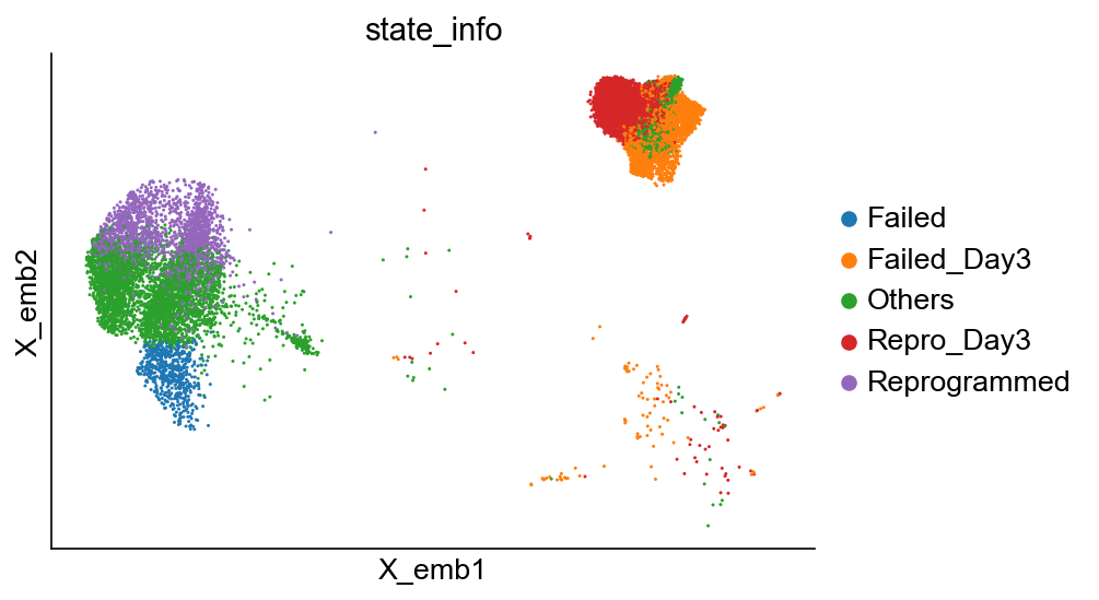
Update cluster annotation on day 3
[45]:
x_emb = adata_1.obsm["X_emb"][:, 0]
state_info = np.array(adata_1.obs["state_info"]).astype(">U15")
sp_idx = (cell_group_A > 0) & (x_emb > 0)
state_info[sp_idx] = "Repro_Day3"

sp_idx = (cell_group_B > 0) & (x_emb > 0)
state_info[sp_idx] = "Failed_Day3"
adata_1.obs["state_info"] = state_info
cs.pl.embedding(adata_1, color="state_info")
/Users/shouwenwang/miniconda3/envs/CoSpar_test/lib/python3.8/site-packages/anndata/_core/anndata.py:1220: FutureWarning: The `inplace` parameter in pandas.Categorical.reorder_categories is deprecated and will be removed in a future version. Reordering categories will always return a new Categorical object.
... storing 'state_info' as categorical
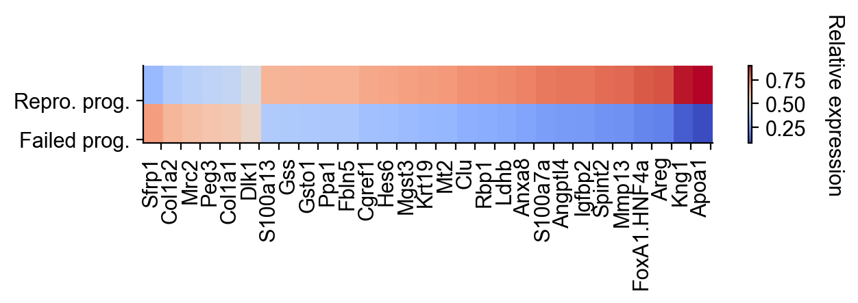
[46]:
cs.settings.set_figure_params(fontsize=12)
gene_list = [
    "FoxA1.HNF4a",
    "Spint2",
    "Apoa1",
    "Hes6",
    "S100a7a",
    "Krt19",
    "Clu",
    "S100a13",
    "Ppa1",
    "Mgst3",
    "Angptl4",
    "Kng1",
    "Igfbp2",
    "Mt2",
    "Areg",
    "Rbp1",
    "Anxa8",
    "Gsto1",
    "Ldhb",
    "Mmp13",
    "Cgref1",
    "Fbln5",
    "Gss",
    "Col1a2",
    "Dlk1",
    "Peg3",
    "Sfrp1",
    "Mrc2",
    "Col1a1",
]

selected_fates = ["Repro_Day3", "Failed_Day3"]
renames = ["Repro. prog.", "Failed prog."]

gene_expression_matrix = cs.pl.gene_expression_heatmap(
    adata_1,
    selected_genes=gene_list,
    selected_fates=selected_fates,
    rename_fates=renames,
    horizontal=True,
    fig_width=6.5,
    fig_height=2,
)
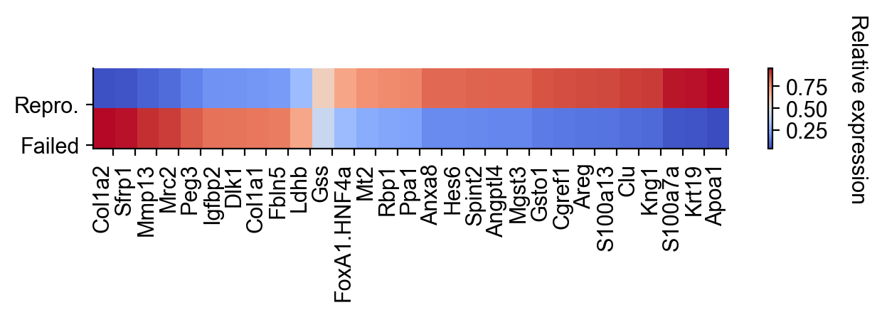
[47]:
gene_list = [
    "FoxA1.HNF4a",
    "Spint2",
    "Apoa1",
    "Hes6",
    "S100a7a",
    "Krt19",
    "Clu",
    "S100a13",
    "Ppa1",
    "Mgst3",
    "Angptl4",
    "Kng1",
    "Igfbp2",
    "Mt2",
    "Areg",
    "Rbp1",
    "Anxa8",
    "Gsto1",
    "Ldhb",
    "Mmp13",
    "Cgref1",
    "Fbln5",
    "Gss",
    "Col1a2",
    "Dlk1",
    "Peg3",
    "Sfrp1",
    "Mrc2",
    "Col1a1",
]

selected_fates = ["Reprogrammed", "Failed"]
renames = ["Repro.", "Failed"]

gene_expression_matrix = cs.pl.gene_expression_heatmap(
    adata_1,
    selected_genes=gene_list,
    selected_fates=selected_fates,
    rename_fates=renames,
    horizontal=True,
    fig_width=6.5,
    fig_height=2,
)